SBML import, observation model, sensitivity analysis, data export and visualization
This is an example using the [model_steadystate_scaled.sbml] model to demonstrate:
SBML import
specifying the observation model
performing sensitivity analysis
exporting and visualizing simulation results
[1]:
# SBML model we want to import
sbml_file = "model_steadystate_scaled_without_observables.xml"
# Name of the model that will also be the name of the python module
model_name = "model_steadystate_scaled"
# Directory to which the generated model code is written
model_output_dir = model_name

import libsbml
import amici
import numpy as np
import matplotlib.pyplot as plt
The example model
Here we use libsbml to show the reactions and species described by the model (this is independent of AMICI).
[2]:
sbml_reader = libsbml.SBMLReader()
sbml_doc = sbml_reader.readSBML(sbml_file)
sbml_model = sbml_doc.getModel()
dir(sbml_doc)

print("Species: ", [s.getId() for s in sbml_model.getListOfSpecies()])

print("\nReactions:")
for reaction in sbml_model.getListOfReactions():
    reactants = " + ".join(
        [
            "%s %s"
            % (
                int(r.getStoichiometry()) if r.getStoichiometry() > 1 else "",
                r.getSpecies(),
            )
            for r in reaction.getListOfReactants()
        ]
    )
    products = " + ".join(
        [
            "%s %s"
            % (
                int(r.getStoichiometry()) if r.getStoichiometry() > 1 else "",
                r.getSpecies(),
            )
            for r in reaction.getListOfProducts()
        ]
    )
    reversible = "<" if reaction.getReversible() else ""
    print(
        "%3s: %10s %1s->%10s\t\t[%s]"
        % (
            reaction.getId(),
            reactants,
            reversible,
            products,
            libsbml.formulaToL3String(reaction.getKineticLaw().getMath()),
        )
    )
Species:  ['x1', 'x2', 'x3']

Reactions:
 r1:       2 x1  ->        x2                [p1 * x1^2]
 r2:   x1 +  x2  ->        x3                [p2 * x1 * x2]
 r3:         x2  ->      2 x1                [p3 * x2]
 r4:         x3  ->  x1 +  x2                [p4 * x3]
 r5:         x3  ->                          [k0 * x3]
 r6:             ->        x1                [p5]
Importing an SBML model, compiling and generating an AMICI module
Before we can use AMICI to simulate our model, the SBML model needs to be translated to C++ code. This is done by amici.SbmlImporter.
[3]:
# Create an SbmlImporter instance for our SBML model
sbml_importer = amici.SbmlImporter(sbml_file)
In this example, we want to specify fixed parameters, observables and a \(\sigma\) parameter. Unfortunately, the latter two are not part of the SBML standard. However, they can be provided to amici.SbmlImporter.sbml2amici as demonstrated in the following.
Constant parameters
Constant parameters, i.e. parameters with respect to which no sensitivities are to be computed (these are often parameters specifying a certain experimental condition) are provided as a list of parameter names.
[4]:
constant_parameters = ["k0"]
Observables
Specifying observables is beyond the scope of SBML. Here we define them manually.
If you are looking for a more scalable way for defining observables, then checkout PEtab. Another possibility is using SBML’s `AssignmentRules <https://sbml.org/software/libsbml/5.18.0/docs/formatted/python-api/classlibsbml_1_1_assignment_rule.html>`__ to specify model outputs within the SBML file.
[5]:
# Define observables
observables = {
    "observable_x1": {"name": "", "formula": "x1"},
    "observable_x2": {"name": "", "formula": "x2"},
    "observable_x3": {"name": "", "formula": "x3"},
    "observable_x1_scaled": {"name": "", "formula": "scaling_x1 * x1"},
    "observable_x2_offsetted": {"name": "", "formula": "offset_x2 + x2"},
    "observable_x1withsigma": {"name": "", "formula": "x1"},
}
\(\sigma\) parameters
To specify measurement noise as a parameter, we simply provide a dictionary with (preexisting) parameter names as keys and a list of observable names as values to indicate which sigma parameter is to be used for which observable.
[6]:
sigmas = {"observable_x1withsigma": "observable_x1withsigma_sigma"}
Generating the module
Now we can generate the python module for our model. amici.SbmlImporter.sbml2amici will symbolically derive the sensitivity equations, generate C++ code for model simulation, and assemble the python module. Standard logging verbosity levels can be passed to this function to see timestamped progression during code generation.
[7]:
import logging

sbml_importer.sbml2amici(
    model_name,
    model_output_dir,
    verbose=logging.INFO,
    observables=observables,
    constant_parameters=constant_parameters,
    sigmas=sigmas,
)
2024-04-23 16:24:35.252 - amici.sbml_import - INFO - Finished importing SBML (6.96E-02s)
2024-04-23 16:24:35.319 - amici.sbml_import - INFO - Finished processing SBML observables (6.10E-02s)
2024-04-23 16:24:35.325 - amici.sbml_import - INFO - Finished processing SBML event observables (1.81E-06s)
2024-04-23 16:24:35.375 - amici.de_model - INFO - Finished computing xdot (7.91E-03s)
2024-04-23 16:24:35.387 - amici.de_model - INFO - Finished computing x0 (6.04E-03s)
2024-04-23 16:24:35.404 - amici.de_model - INFO - Finished computing w (1.06E-02s)
2024-04-23 16:24:36.621 - amici.de_export - INFO - Finished generating cpp code (1.21E+00s)
2024-04-23 16:24:54.927 - amici.de_export - INFO - Finished compiling cpp code (1.83E+01s)
Importing the module and loading the model
If everything went well, we can now import the newly generated Python module containing our model:
[8]:
model_module = amici.import_model_module(model_name, model_output_dir)
And get an instance of our model from which we can retrieve information such as parameter names:
[9]:
model = model_module.getModel()

print("Model name:      ", model.getName())
print("Model parameters:", model.getParameterIds())
print("Model outputs:   ", model.getObservableIds())
print("Model states:    ", model.getStateIds())
Model name:       model_steadystate_scaled
Model parameters: ('p1', 'p2', 'p3', 'p4', 'p5', 'scaling_x1', 'offset_x2', 'observable_x1withsigma_sigma')
Model outputs:    ('observable_x1', 'observable_x2', 'observable_x3', 'observable_x1_scaled', 'observable_x2_offsetted', 'observable_x1withsigma')
Model states:     ('x1', 'x2', 'x3')
Running simulations and analyzing results
After importing the model, we can run simulations using amici.runAmiciSimulation. This requires a Model instance and a Solver instance. Optionally you can provide measurements inside an ExpData instance, as shown later in this notebook.
[10]:
# Create Model instance
model = model_module.getModel()

# set timepoints for which we want to simulate the model
model.setTimepoints(np.linspace(0, 60, 60))

# Create solver instance
solver = model.getSolver()

# Run simulation using default model parameters and solver options
rdata = amici.runAmiciSimulation(model, solver)
[11]:
print(
    "Simulation was run using model default parameters as specified in the SBML model:"
)
print(dict(zip(model.getParameterIds(), model.getParameters())))
Simulation was run using model default parameters as specified in the SBML model:
{'p1': 1.0, 'p2': 0.5, 'p3': 0.4, 'p4': 2.0, 'p5': 0.1, 'scaling_x1': 2.0, 'offset_x2': 3.0, 'observable_x1withsigma_sigma': 0.2}
Simulation results are provided as numpy.ndarrays in the returned dictionary:
[12]:
# np.set_printoptions(threshold=8, edgeitems=2)
for key, value in rdata.items():
    print("%12s: " % key, value)
          ts:  [ 0.          1.01694915  2.03389831  3.05084746  4.06779661  5.08474576
  6.10169492  7.11864407  8.13559322  9.15254237 10.16949153 11.18644068
 12.20338983 13.22033898 14.23728814 15.25423729 16.27118644 17.28813559
 18.30508475 19.3220339  20.33898305 21.3559322  22.37288136 23.38983051
 24.40677966 25.42372881 26.44067797 27.45762712 28.47457627 29.49152542
 30.50847458 31.52542373 32.54237288 33.55932203 34.57627119 35.59322034
 36.61016949 37.62711864 38.6440678  39.66101695 40.6779661  41.69491525
 42.71186441 43.72881356 44.74576271 45.76271186 46.77966102 47.79661017
 48.81355932 49.83050847 50.84745763 51.86440678 52.88135593 53.89830508
 54.91525424 55.93220339 56.94915254 57.96610169 58.98305085 60.        ]
           x:  [[0.1        0.4        0.7       ]
 [0.57995052 0.73365809 0.0951589 ]
 [0.55996496 0.71470091 0.0694127 ]
 [0.5462855  0.68030366 0.06349394]
 [0.53561883 0.64937432 0.05923555]
 [0.52636487 0.62259567 0.05568686]
 [0.51822013 0.59943346 0.05268079]
 [0.51103767 0.57935661 0.05012037]
 [0.5047003  0.56191592 0.04793052]
 [0.49910666 0.54673518 0.0460508 ]
 [0.49416809 0.53349812 0.04443205]
 [0.48980687 0.52193767 0.04303399]
 [0.48595476 0.51182731 0.04182339]
 [0.48255176 0.50297412 0.04077267]
 [0.47954511 0.49521318 0.03985882]
 [0.47688833 0.48840304 0.03906254]
 [0.47454049 0.48242198 0.03836756]
 [0.47246548 0.47716502 0.0377601 ]
 [0.47063147 0.47254128 0.03722844]
 [0.46901037 0.46847202 0.03676259]
 [0.46757739 0.46488881 0.03635397]
 [0.46631065 0.46173207 0.03599523]
 [0.46519082 0.45894987 0.03568002]
 [0.46420083 0.45649684 0.03540285]
 [0.4633256  0.45433332 0.03515899]
 [0.4625518  0.45242457 0.03494429]
 [0.46186768 0.45074016 0.03475519]
 [0.46126282 0.44925337 0.03458856]
 [0.46072804 0.44794075 0.03444166]
 [0.46025521 0.44678168 0.03431212]
 [0.45983714 0.44575804 0.03419784]
 [0.45946749 0.44485388 0.03409701]
 [0.45914065 0.44405514 0.03400802]
 [0.45885167 0.44334947 0.03392946]
 [0.45859615 0.44272595 0.03386009]
 [0.45837021 0.44217497 0.03379883]
 [0.45817043 0.44168805 0.03374473]
 [0.45799379 0.44125772 0.03369693]
 [0.4578376  0.44087738 0.03365471]
 [0.45769949 0.44054121 0.0336174 ]
 [0.45757737 0.44024405 0.03358444]
 [0.45746939 0.43998137 0.03355531]
 [0.45737391 0.43974917 0.03352956]
 [0.45728948 0.43954389 0.03350681]
 [0.45721483 0.43936242 0.0334867 ]
 [0.45714882 0.43920198 0.03346892]
 [0.45709045 0.43906014 0.03345321]
 [0.45703884 0.43893474 0.03343932]
 [0.4569932  0.43882387 0.03342704]
 [0.45695285 0.43872584 0.03341618]
 [0.45691717 0.43863917 0.03340658]
 [0.45688561 0.43856254 0.0333981 ]
 [0.45685771 0.43849478 0.0333906 ]
 [0.45683304 0.43843488 0.03338397]
 [0.45681123 0.4383819  0.0333781 ]
 [0.45679194 0.43833507 0.03337292]
 [0.45677488 0.43829365 0.03336833]
 [0.4567598  0.43825703 0.03336428]
 [0.45674646 0.43822466 0.0333607 ]
 [0.45673467 0.43819603 0.03335753]]
          x0:  [0.1 0.4 0.7]
        x_ss:  [nan nan nan]
          sx:  None
         sx0:  None
       sx_ss:  None
           y:  [[0.1        0.4        0.7        0.2        3.4        0.1       ]
 [0.57995052 0.73365809 0.0951589  1.15990103 3.73365809 0.57995052]
 [0.55996496 0.71470091 0.0694127  1.11992992 3.71470091 0.55996496]
 [0.5462855  0.68030366 0.06349394 1.092571   3.68030366 0.5462855 ]
 [0.53561883 0.64937432 0.05923555 1.07123766 3.64937432 0.53561883]
 [0.52636487 0.62259567 0.05568686 1.05272975 3.62259567 0.52636487]
 [0.51822013 0.59943346 0.05268079 1.03644027 3.59943346 0.51822013]
 [0.51103767 0.57935661 0.05012037 1.02207533 3.57935661 0.51103767]
 [0.5047003  0.56191592 0.04793052 1.00940059 3.56191592 0.5047003 ]
 [0.49910666 0.54673518 0.0460508  0.99821331 3.54673518 0.49910666]
 [0.49416809 0.53349812 0.04443205 0.98833618 3.53349812 0.49416809]
 [0.48980687 0.52193767 0.04303399 0.97961374 3.52193767 0.48980687]
 [0.48595476 0.51182731 0.04182339 0.97190952 3.51182731 0.48595476]
 [0.48255176 0.50297412 0.04077267 0.96510352 3.50297412 0.48255176]
 [0.47954511 0.49521318 0.03985882 0.95909022 3.49521318 0.47954511]
 [0.47688833 0.48840304 0.03906254 0.95377667 3.48840304 0.47688833]
 [0.47454049 0.48242198 0.03836756 0.94908097 3.48242198 0.47454049]
 [0.47246548 0.47716502 0.0377601  0.94493095 3.47716502 0.47246548]
 [0.47063147 0.47254128 0.03722844 0.94126293 3.47254128 0.47063147]
 [0.46901037 0.46847202 0.03676259 0.93802074 3.46847202 0.46901037]
 [0.46757739 0.46488881 0.03635397 0.93515478 3.46488881 0.46757739]
 [0.46631065 0.46173207 0.03599523 0.9326213  3.46173207 0.46631065]
 [0.46519082 0.45894987 0.03568002 0.93038164 3.45894987 0.46519082]
 [0.46420083 0.45649684 0.03540285 0.92840166 3.45649684 0.46420083]
 [0.4633256  0.45433332 0.03515899 0.92665119 3.45433332 0.4633256 ]
 [0.4625518  0.45242457 0.03494429 0.9251036  3.45242457 0.4625518 ]
 [0.46186768 0.45074016 0.03475519 0.92373536 3.45074016 0.46186768]
 [0.46126282 0.44925337 0.03458856 0.92252564 3.44925337 0.46126282]
 [0.46072804 0.44794075 0.03444166 0.92145608 3.44794075 0.46072804]
 [0.46025521 0.44678168 0.03431212 0.92051041 3.44678168 0.46025521]
 [0.45983714 0.44575804 0.03419784 0.91967427 3.44575804 0.45983714]
 [0.45946749 0.44485388 0.03409701 0.91893498 3.44485388 0.45946749]
 [0.45914065 0.44405514 0.03400802 0.91828131 3.44405514 0.45914065]
 [0.45885167 0.44334947 0.03392946 0.91770333 3.44334947 0.45885167]
 [0.45859615 0.44272595 0.03386009 0.91719229 3.44272595 0.45859615]
 [0.45837021 0.44217497 0.03379883 0.91674042 3.44217497 0.45837021]
 [0.45817043 0.44168805 0.03374473 0.91634087 3.44168805 0.45817043]
 [0.45799379 0.44125772 0.03369693 0.91598758 3.44125772 0.45799379]
 [0.4578376  0.44087738 0.03365471 0.9156752  3.44087738 0.4578376 ]
 [0.45769949 0.44054121 0.0336174  0.91539898 3.44054121 0.45769949]
 [0.45757737 0.44024405 0.03358444 0.91515474 3.44024405 0.45757737]
 [0.45746939 0.43998137 0.03355531 0.91493878 3.43998137 0.45746939]
 [0.45737391 0.43974917 0.03352956 0.91474782 3.43974917 0.45737391]
 [0.45728948 0.43954389 0.03350681 0.91457897 3.43954389 0.45728948]
 [0.45721483 0.43936242 0.0334867  0.91442966 3.43936242 0.45721483]
 [0.45714882 0.43920198 0.03346892 0.91429764 3.43920198 0.45714882]
 [0.45709045 0.43906014 0.03345321 0.91418091 3.43906014 0.45709045]
 [0.45703884 0.43893474 0.03343932 0.91407768 3.43893474 0.45703884]
 [0.4569932  0.43882387 0.03342704 0.91398641 3.43882387 0.4569932 ]
 [0.45695285 0.43872584 0.03341618 0.9139057  3.43872584 0.45695285]
 [0.45691717 0.43863917 0.03340658 0.91383433 3.43863917 0.45691717]
 [0.45688561 0.43856254 0.0333981  0.91377123 3.43856254 0.45688561]
 [0.45685771 0.43849478 0.0333906  0.91371543 3.43849478 0.45685771]
 [0.45683304 0.43843488 0.03338397 0.91366609 3.43843488 0.45683304]
 [0.45681123 0.4383819  0.0333781  0.91362246 3.4383819  0.45681123]
 [0.45679194 0.43833507 0.03337292 0.91358388 3.43833507 0.45679194]
 [0.45677488 0.43829365 0.03336833 0.91354976 3.43829365 0.45677488]
 [0.4567598  0.43825703 0.03336428 0.9135196  3.43825703 0.4567598 ]
 [0.45674646 0.43822466 0.0333607  0.91349292 3.43822466 0.45674646]
 [0.45673467 0.43819603 0.03335753 0.91346934 3.43819603 0.45673467]]
      sigmay:  [[1.  1.  1.  1.  1.  0.2]
 [1.  1.  1.  1.  1.  0.2]
 [1.  1.  1.  1.  1.  0.2]
 [1.  1.  1.  1.  1.  0.2]
 [1.  1.  1.  1.  1.  0.2]
 [1.  1.  1.  1.  1.  0.2]
 [1.  1.  1.  1.  1.  0.2]
 [1.  1.  1.  1.  1.  0.2]
 [1.  1.  1.  1.  1.  0.2]
 [1.  1.  1.  1.  1.  0.2]
 [1.  1.  1.  1.  1.  0.2]
 [1.  1.  1.  1.  1.  0.2]
 [1.  1.  1.  1.  1.  0.2]
 [1.  1.  1.  1.  1.  0.2]
 [1.  1.  1.  1.  1.  0.2]
 [1.  1.  1.  1.  1.  0.2]
 [1.  1.  1.  1.  1.  0.2]
 [1.  1.  1.  1.  1.  0.2]
 [1.  1.  1.  1.  1.  0.2]
 [1.  1.  1.  1.  1.  0.2]
 [1.  1.  1.  1.  1.  0.2]
 [1.  1.  1.  1.  1.  0.2]
 [1.  1.  1.  1.  1.  0.2]
 [1.  1.  1.  1.  1.  0.2]
 [1.  1.  1.  1.  1.  0.2]
 [1.  1.  1.  1.  1.  0.2]
 [1.  1.  1.  1.  1.  0.2]
 [1.  1.  1.  1.  1.  0.2]
 [1.  1.  1.  1.  1.  0.2]
 [1.  1.  1.  1.  1.  0.2]
 [1.  1.  1.  1.  1.  0.2]
 [1.  1.  1.  1.  1.  0.2]
 [1.  1.  1.  1.  1.  0.2]
 [1.  1.  1.  1.  1.  0.2]
 [1.  1.  1.  1.  1.  0.2]
 [1.  1.  1.  1.  1.  0.2]
 [1.  1.  1.  1.  1.  0.2]
 [1.  1.  1.  1.  1.  0.2]
 [1.  1.  1.  1.  1.  0.2]
 [1.  1.  1.  1.  1.  0.2]
 [1.  1.  1.  1.  1.  0.2]
 [1.  1.  1.  1.  1.  0.2]
 [1.  1.  1.  1.  1.  0.2]
 [1.  1.  1.  1.  1.  0.2]
 [1.  1.  1.  1.  1.  0.2]
 [1.  1.  1.  1.  1.  0.2]
 [1.  1.  1.  1.  1.  0.2]
 [1.  1.  1.  1.  1.  0.2]
 [1.  1.  1.  1.  1.  0.2]
 [1.  1.  1.  1.  1.  0.2]
 [1.  1.  1.  1.  1.  0.2]
 [1.  1.  1.  1.  1.  0.2]
 [1.  1.  1.  1.  1.  0.2]
 [1.  1.  1.  1.  1.  0.2]
 [1.  1.  1.  1.  1.  0.2]
 [1.  1.  1.  1.  1.  0.2]
 [1.  1.  1.  1.  1.  0.2]
 [1.  1.  1.  1.  1.  0.2]
 [1.  1.  1.  1.  1.  0.2]
 [1.  1.  1.  1.  1.  0.2]]
          sy:  None
     ssigmay:  None
           z:  None
          rz:  None
      sigmaz:  None
          sz:  None
         srz:  None
     ssigmaz:  None
        sllh:  None
       s2llh:  None
           J:  [[-2.04603669  0.57163267  2.        ]
 [ 0.69437133 -0.62836733  2.        ]
 [ 0.21909801  0.22836733 -3.        ]]
        xdot:  [-1.08967281e-05 -2.64534209e-05 -2.92761862e-06]
      status:  0
         llh:  nan
        chi2:  nan
         res:  [0. 0. 0. 0. 0. 0. 0. 0. 0. 0. 0. 0. 0. 0. 0. 0. 0. 0. 0. 0. 0. 0. 0. 0.
 0. 0. 0. 0. 0. 0. 0. 0. 0. 0. 0. 0. 0. 0. 0. 0. 0. 0. 0. 0. 0. 0. 0. 0.
 0. 0. 0. 0. 0. 0. 0. 0. 0. 0. 0. 0. 0. 0. 0. 0. 0. 0. 0. 0. 0. 0. 0. 0.
 0. 0. 0. 0. 0. 0. 0. 0. 0. 0. 0. 0. 0. 0. 0. 0. 0. 0. 0. 0. 0. 0. 0. 0.
 0. 0. 0. 0. 0. 0. 0. 0. 0. 0. 0. 0. 0. 0. 0. 0. 0. 0. 0. 0. 0. 0. 0. 0.
 0. 0. 0. 0. 0. 0. 0. 0. 0. 0. 0. 0. 0. 0. 0. 0. 0. 0. 0. 0. 0. 0. 0. 0.
 0. 0. 0. 0. 0. 0. 0. 0. 0. 0. 0. 0. 0. 0. 0. 0. 0. 0. 0. 0. 0. 0. 0. 0.
 0. 0. 0. 0. 0. 0. 0. 0. 0. 0. 0. 0. 0. 0. 0. 0. 0. 0. 0. 0. 0. 0. 0. 0.
 0. 0. 0. 0. 0. 0. 0. 0. 0. 0. 0. 0. 0. 0. 0. 0. 0. 0. 0. 0. 0. 0. 0. 0.
 0. 0. 0. 0. 0. 0. 0. 0. 0. 0. 0. 0. 0. 0. 0. 0. 0. 0. 0. 0. 0. 0. 0. 0.
 0. 0. 0. 0. 0. 0. 0. 0. 0. 0. 0. 0. 0. 0. 0. 0. 0. 0. 0. 0. 0. 0. 0. 0.
 0. 0. 0. 0. 0. 0. 0. 0. 0. 0. 0. 0. 0. 0. 0. 0. 0. 0. 0. 0. 0. 0. 0. 0.
 0. 0. 0. 0. 0. 0. 0. 0. 0. 0. 0. 0. 0. 0. 0. 0. 0. 0. 0. 0. 0. 0. 0. 0.
 0. 0. 0. 0. 0. 0. 0. 0. 0. 0. 0. 0. 0. 0. 0. 0. 0. 0. 0. 0. 0. 0. 0. 0.
 0. 0. 0. 0. 0. 0. 0. 0. 0. 0. 0. 0. 0. 0. 0. 0. 0. 0. 0. 0. 0. 0. 0. 0.]
        sres:  None
         FIM:  None
           w:  [[0.01       0.02       0.16       1.4        0.7        0.1       ]
 [0.3363426  0.21274269 0.29346324 0.1903178  0.0951589  0.1       ]
 [0.31356076 0.20010373 0.28588036 0.13882541 0.0694127  0.1       ]
 [0.29842785 0.18582001 0.27212146 0.12698788 0.06349394 0.1       ]
 [0.28688753 0.17390856 0.25974973 0.1184711  0.05923555 0.1       ]
 [0.27705998 0.16385625 0.24903827 0.11137372 0.05568686 0.1       ]
 [0.26855211 0.15531924 0.23977338 0.10536158 0.05268079 0.1       ]
 [0.2611595  0.14803652 0.23174264 0.10024074 0.05012037 0.1       ]
 [0.25472239 0.14179957 0.22476637 0.09586103 0.04793052 0.1       ]
 [0.24910746 0.13643958 0.21869407 0.0921016  0.0460508  0.1       ]
 [0.2442021  0.13181887 0.21339925 0.08886411 0.04443205 0.1       ]
 [0.23991077 0.12782433 0.20877507 0.08606799 0.04303399 0.1       ]
 [0.23615203 0.12436246 0.20473093 0.08364678 0.04182339 0.1       ]
 [0.2328562  0.12135552 0.20118965 0.08154533 0.04077267 0.1       ]
 [0.22996351 0.11873853 0.19808527 0.07971763 0.03985882 0.1       ]
 [0.22742248 0.11645686 0.19536122 0.07812507 0.03906254 0.1       ]
 [0.22518867 0.11446438 0.19296879 0.07673511 0.03836756 0.1       ]
 [0.22322363 0.112722   0.19086601 0.0755202  0.0377601  0.1       ]
 [0.22149398 0.1111964  0.18901651 0.07445688 0.03722844 0.1       ]
 [0.21997073 0.10985912 0.18738881 0.07352518 0.03676259 0.1       ]
 [0.21862862 0.10868575 0.18595552 0.07270794 0.03635397 0.1       ]
 [0.21744562 0.10765529 0.18469283 0.07199046 0.03599523 0.1       ]
 [0.2164025  0.10674963 0.18357995 0.07136003 0.03568002 0.1       ]
 [0.21548241 0.10595311 0.18259874 0.0708057  0.03540285 0.1       ]
 [0.21467061 0.10525213 0.18173333 0.07031797 0.03515899 0.1       ]
 [0.21395417 0.1046349  0.18096983 0.06988859 0.03494429 0.1       ]
 [0.21332175 0.10409116 0.18029606 0.06951039 0.03475519 0.1       ]
 [0.21276339 0.10361194 0.17970135 0.06917712 0.03458856 0.1       ]
 [0.21227033 0.10318943 0.1791763  0.06888332 0.03444166 0.1       ]
 [0.21183485 0.1028168  0.17871267 0.06862424 0.03431212 0.1       ]
 [0.21145019 0.10248805 0.17830322 0.06839569 0.03419784 0.1       ]
 [0.21111037 0.10219795 0.17794155 0.06819402 0.03409701 0.1       ]
 [0.21081014 0.10194188 0.17762206 0.06801603 0.03400802 0.1       ]
 [0.21054485 0.10171582 0.17733979 0.06785891 0.03392946 0.1       ]
 [0.21031042 0.10151621 0.17709038 0.06772018 0.03386009 0.1       ]
 [0.21010325 0.10133992 0.17686999 0.06759766 0.03379883 0.1       ]
 [0.20992015 0.1011842  0.17667522 0.06748945 0.03374473 0.1       ]
 [0.20975831 0.10104665 0.17650309 0.06739386 0.03369693 0.1       ]
 [0.20961527 0.10092512 0.17635095 0.06730942 0.03365471 0.1       ]
 [0.20948882 0.10081774 0.17621648 0.0672348  0.0336174  0.1       ]
 [0.20937705 0.10072286 0.17609762 0.06716887 0.03358444 0.1       ]
 [0.20927824 0.10063901 0.17599255 0.06711061 0.03355531 0.1       ]
 [0.20919089 0.1005649  0.17589967 0.06705912 0.03352956 0.1       ]
 [0.20911367 0.1004994  0.17581756 0.06701361 0.03350681 0.1       ]
 [0.2090454  0.10044151 0.17574497 0.06697339 0.0334867  0.1       ]
 [0.20898505 0.10039033 0.17568079 0.06693784 0.03346892 0.1       ]
 [0.20893168 0.1003451  0.17562406 0.06690641 0.03345321 0.1       ]
 [0.2088845  0.10030511 0.1755739  0.06687863 0.03343932 0.1       ]
 [0.20884279 0.10026976 0.17552955 0.06685407 0.03342704 0.1       ]
 [0.20880591 0.10023851 0.17549034 0.06683236 0.03341618 0.1       ]
 [0.2087733  0.10021088 0.17545567 0.06681317 0.03340658 0.1       ]
 [0.20874446 0.10018646 0.17542502 0.0667962  0.0333981  0.1       ]
 [0.20871897 0.10016486 0.17539791 0.0667812  0.0333906  0.1       ]
 [0.20869643 0.10014577 0.17537395 0.06676793 0.03338397 0.1       ]
 [0.2086765  0.10012889 0.17535276 0.0667562  0.0333781  0.1       ]
 [0.20865887 0.10011396 0.17533403 0.06674583 0.03337292 0.1       ]
 [0.20864329 0.10010077 0.17531746 0.06673667 0.03336833 0.1       ]
 [0.20862951 0.1000891  0.17530281 0.06672856 0.03336428 0.1       ]
 [0.20861733 0.10007878 0.17528986 0.06672139 0.0333607  0.1       ]
 [0.20860656 0.10006966 0.17527841 0.06671506 0.03335753 0.1       ]]
  preeq_wrms:  nan
     preeq_t:  nan
preeq_numsteps:  [[0 0 0]]
preeq_numstepsB:  0.0
preeq_status:  [[0 0 0]]
preeq_cpu_time:  0.0
preeq_cpu_timeB:  0.0
 posteq_wrms:  nan
    posteq_t:  nan
posteq_numsteps:  [[0 0 0]]
posteq_numstepsB:  0.0
posteq_status:  [[0 0 0]]
posteq_cpu_time:  0.0
posteq_cpu_timeB:  0.0
    numsteps:  [  0 100 144 165 181 191 200 207 213 218 223 228 233 237 241 245 249 252
 255 258 261 264 266 269 272 275 278 282 286 290 293 296 299 303 307 311
 314 317 321 325 328 333 337 340 342 344 346 348 350 352 354 356 358 359
 360 361 362 363 364 365]
 numrhsevals:  [  0 114 160 193 212 227 237 248 255 260 267 272 277 282 287 292 296 300
 303 306 309 312 315 318 322 325 329 333 337 342 345 348 352 358 365 369
 372 376 381 385 389 395 400 403 405 407 409 411 413 415 417 419 421 422
 424 426 427 428 429 430]
numerrtestfails:  [0 1 1 3 3 4 4 5 5 5 5 5 5 5 5 5 5 5 5 5 5 5 5 5 5 5 5 5 5 5 5 5 5 5 6 6 6
 6 6 6 6 6 6 6 6 6 6 6 6 6 6 6 6 6 6 6 6 6 6 6]
numnonlinsolvconvfails:  [0 0 0 0 0 0 0 0 0 0 0 0 0 0 0 0 0 0 0 0 0 0 0 0 0 0 0 0 0 0 0 0 0 0 0 0 0
 0 0 0 0 0 0 0 0 0 0 0 0 0 0 0 0 0 0 0 0 0 0 0]
       order:  [0 5 5 5 5 5 4 5 4 5 4 4 4 4 4 4 5 5 5 5 5 5 5 5 4 4 5 5 5 4 4 4 5 5 5 4 4
 4 4 5 5 4 5 5 5 5 5 5 5 4 4 4 4 4 4 4 4 4 4 4]
    cpu_time:  1.3669999999999976
   numstepsB:  None
numrhsevalsB:  None
numerrtestfailsB:  None
numnonlinsolvconvfailsB:  None
   cpu_timeB:  0.0
cpu_time_total:  1.919
    messages:  <Swig Object of type 'std::vector< amici::LogItem > *' at 0x7f02aee838a0; [] >
      t_last:  60.0
[13]:
# In particular for interactive use, ReturnDataView.by_id() and amici.evaluate provides a more convenient way to access slices of the result:
# Time trajectory of observable observable_x1
print(f"{rdata.by_id('observable_x1')=}")
# Time trajectory of state variable x2
print(f"{rdata.by_id('x2')=}")
rdata.by_id('observable_x1')=array([0.1       , 0.57995052, 0.55996496, 0.5462855 , 0.53561883,
       0.52636487, 0.51822013, 0.51103767, 0.5047003 , 0.49910666,
       0.49416809, 0.48980687, 0.48595476, 0.48255176, 0.47954511,
       0.47688833, 0.47454049, 0.47246548, 0.47063147, 0.46901037,
       0.46757739, 0.46631065, 0.46519082, 0.46420083, 0.4633256 ,
       0.4625518 , 0.46186768, 0.46126282, 0.46072804, 0.46025521,
       0.45983714, 0.45946749, 0.45914065, 0.45885167, 0.45859615,
       0.45837021, 0.45817043, 0.45799379, 0.4578376 , 0.45769949,
       0.45757737, 0.45746939, 0.45737391, 0.45728948, 0.45721483,
       0.45714882, 0.45709045, 0.45703884, 0.4569932 , 0.45695285,
       0.45691717, 0.45688561, 0.45685771, 0.45683304, 0.45681123,
       0.45679194, 0.45677488, 0.4567598 , 0.45674646, 0.45673467])
rdata.by_id('x2')=array([0.4       , 0.73365809, 0.71470091, 0.68030366, 0.64937432,
       0.62259567, 0.59943346, 0.57935661, 0.56191592, 0.54673518,
       0.53349812, 0.52193767, 0.51182731, 0.50297412, 0.49521318,
       0.48840304, 0.48242198, 0.47716502, 0.47254128, 0.46847202,
       0.46488881, 0.46173207, 0.45894987, 0.45649684, 0.45433332,
       0.45242457, 0.45074016, 0.44925337, 0.44794075, 0.44678168,
       0.44575804, 0.44485388, 0.44405514, 0.44334947, 0.44272595,
       0.44217497, 0.44168805, 0.44125772, 0.44087738, 0.44054121,
       0.44024405, 0.43998137, 0.43974917, 0.43954389, 0.43936242,
       0.43920198, 0.43906014, 0.43893474, 0.43882387, 0.43872584,
       0.43863917, 0.43856254, 0.43849478, 0.43843488, 0.4383819 ,
       0.43833507, 0.43829365, 0.43825703, 0.43822466, 0.43819603])
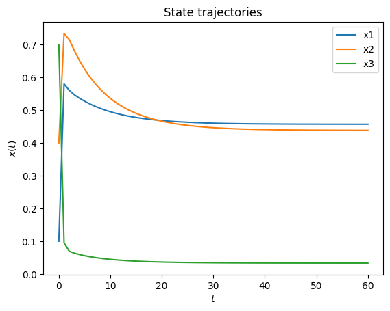
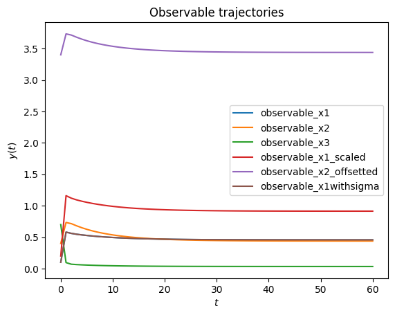
Plotting trajectories
The simulation results above did not look too appealing. Let’s plot the trajectories of the model states and outputs them using matplotlib.pyplot:
[14]:
import amici.plotting

amici.plotting.plot_state_trajectories(rdata, model=None)
amici.plotting.plot_observable_trajectories(rdata, model=None)
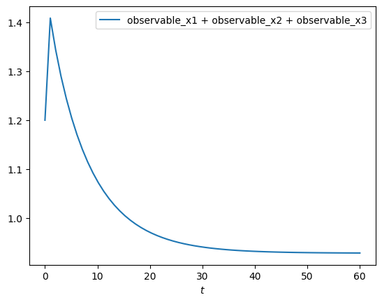
We can also evaluate symbolic expressions of model quantities using amici.numpy.evaluate, or directly plot the results using amici.plotting.plot_expressions:
[15]:
amici.plotting.plot_expressions(
    "observable_x1 + observable_x2 + observable_x3", rdata=rdata
)
Computing likelihood
Often model parameters need to be inferred from experimental data. This is commonly done by maximizing the likelihood of observing the data given to current model parameters. AMICI will compute this likelihood if experimental data is provided to amici.runAmiciSimulation as optional third argument. Measurements along with their standard deviations are provided through an amici.ExpData instance.
[16]:
# Create model instance and set time points for simulation
model = model_module.getModel()
model.setTimepoints(np.linspace(0, 10, 11))

# Create solver instance, keep default options
solver = model.getSolver()

# Run simulation without experimental data
rdata = amici.runAmiciSimulation(model, solver)

# Create ExpData instance from simulation results
edata = amici.ExpData(rdata, 1.0, 0.0)

# Re-run simulation, this time passing "experimental data"
rdata = amici.runAmiciSimulation(model, solver, edata)

print("Log-likelihood %f" % rdata["llh"])
Log-likelihood -99.675431
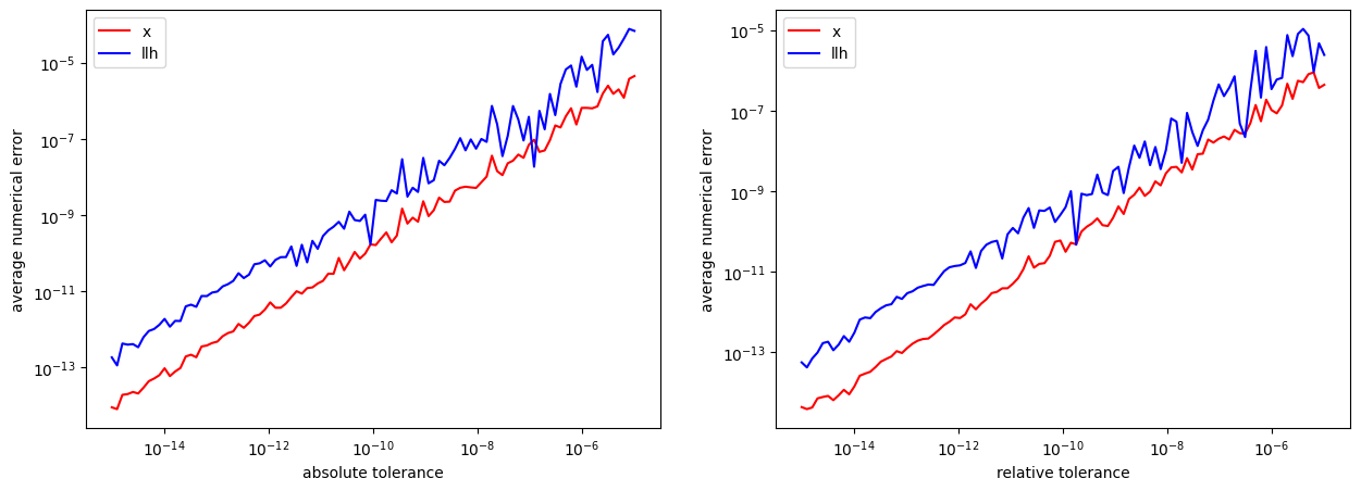
Simulation tolerances
Numerical error tolerances are often critical to get accurate results. For the state variables, integration errors can be controlled using setRelativeTolerance and setAbsoluteTolerance. Similar functions exist for sensitivities, steadystates and quadratures. We initially compute a reference solution using extremely low tolerances and then assess the influence on integration error for different levels of absolute and relative tolerance.
[17]:
solver.setRelativeTolerance(1e-16)
solver.setAbsoluteTolerance(1e-16)
solver.setSensitivityOrder(amici.SensitivityOrder.none)
rdata_ref = amici.runAmiciSimulation(model, solver, edata)


def get_simulation_error(solver):
    rdata = amici.runAmiciSimulation(model, solver, edata)
    return np.mean(np.abs(rdata["x"] - rdata_ref["x"])), np.mean(
        np.abs(rdata["llh"] - rdata_ref["llh"])
    )


def get_errors(tolfun, tols):
    solver.setRelativeTolerance(1e-16)
    solver.setAbsoluteTolerance(1e-16)
    x_errs = []
    llh_errs = []
    for tol in tols:
        getattr(solver, tolfun)(tol)
        x_err, llh_err = get_simulation_error(solver)
        x_errs.append(x_err)
        llh_errs.append(llh_err)
    return x_errs, llh_errs


atols = np.logspace(-5, -15, 100)
atol_x_errs, atol_llh_errs = get_errors("setAbsoluteTolerance", atols)

rtols = np.logspace(-5, -15, 100)
rtol_x_errs, rtol_llh_errs = get_errors("setRelativeTolerance", rtols)

fig, axes = plt.subplots(1, 2, figsize=(15, 5))


def plot_error(tols, x_errs, llh_errs, tolname, ax):
    ax.plot(tols, x_errs, "r-", label="x")
    ax.plot(tols, llh_errs, "b-", label="llh")
    ax.set_xscale("log")
    ax.set_yscale("log")
    ax.set_xlabel(f"{tolname} tolerance")
    ax.set_ylabel("average numerical error")
    ax.legend()


plot_error(atols, atol_x_errs, atol_llh_errs, "absolute", axes[0])
plot_error(rtols, rtol_x_errs, rtol_llh_errs, "relative", axes[1])

# reset relative tolerance to default value
solver.setRelativeTolerance(1e-8)
solver.setRelativeTolerance(1e-16)
Sensitivity analysis
AMICI can provide first- and second-order sensitivities using the forward- or adjoint-method. The respective options are set on the Model and Solver objects.
Forward sensitivity analysis
[18]:
model = model_module.getModel()
model.setTimepoints(np.linspace(0, 10, 11))
model.requireSensitivitiesForAllParameters()  # sensitivities w.r.t. all parameters
# model.setParameterList([1, 2])                          # sensitivities
# w.r.t. the specified parameters
model.setParameterScale(
    amici.ParameterScaling.none
)  # parameters are used as-is (not log-transformed)

solver = model.getSolver()
solver.setSensitivityMethod(
    amici.SensitivityMethod.forward
)  # forward sensitivity analysis
solver.setSensitivityOrder(
    amici.SensitivityOrder.first
)  # first-order sensitivities

rdata = amici.runAmiciSimulation(model, solver)

# print sensitivity-related results
for key, value in rdata.items():
    if key.startswith("s"):
        print("%12s: " % key, value)
          sx:  [[[ 0.00000000e+00  0.00000000e+00  0.00000000e+00]
  [ 0.00000000e+00  0.00000000e+00  0.00000000e+00]
  [ 0.00000000e+00  0.00000000e+00  0.00000000e+00]
  [ 0.00000000e+00  0.00000000e+00  0.00000000e+00]
  [ 0.00000000e+00  0.00000000e+00  0.00000000e+00]
  [ 0.00000000e+00  0.00000000e+00  0.00000000e+00]
  [ 0.00000000e+00  0.00000000e+00  0.00000000e+00]
  [ 0.00000000e+00  0.00000000e+00  0.00000000e+00]]

 [[-2.00747250e-01  1.19873139e-01 -9.44167985e-03]
  [-1.02561396e-01 -1.88820454e-01  1.01855972e-01]
  [ 4.66193077e-01 -2.86365372e-01  2.39662449e-02]
  [ 4.52560294e-02  1.14631370e-01 -3.34067919e-02]
  [ 4.00672911e-01  1.92564093e-01  4.98877759e-02]
  [ 0.00000000e+00  0.00000000e+00  0.00000000e+00]
  [ 0.00000000e+00  0.00000000e+00  0.00000000e+00]
  [ 0.00000000e+00  0.00000000e+00  0.00000000e+00]]

 [[-2.23007240e-01  1.53979022e-01 -1.26885280e-02]
  [-1.33426939e-01 -3.15955239e-01  9.49575030e-02]
  [ 5.03470377e-01 -3.52731535e-01  2.81567412e-02]
  [ 3.93630714e-02  1.10770683e-01 -1.05673869e-02]
  [ 5.09580304e-01  4.65255489e-01  9.24843702e-02]
  [ 0.00000000e+00  0.00000000e+00  0.00000000e+00]
  [ 0.00000000e+00  0.00000000e+00  0.00000000e+00]
  [ 0.00000000e+00  0.00000000e+00  0.00000000e+00]]

 [[-2.14278104e-01  1.63465064e-01 -1.03268418e-02]
  [-1.60981967e-01 -4.00490452e-01  7.54810648e-02]
  [ 4.87746419e-01 -3.76014315e-01  2.30919334e-02]
  [ 4.28733680e-02  1.15473583e-01 -6.63571687e-03]
  [ 6.05168647e-01  7.07226039e-01  1.23870914e-01]
  [ 0.00000000e+00  0.00000000e+00  0.00000000e+00]
  [ 0.00000000e+00  0.00000000e+00  0.00000000e+00]
  [ 0.00000000e+00  0.00000000e+00  0.00000000e+00]]

 [[-2.05888038e-01  1.69308689e-01 -7.93085660e-03]
  [-1.84663809e-01 -4.65451966e-01  5.95026117e-02]
  [ 4.66407064e-01 -3.87612079e-01  1.76410128e-02]
  [ 4.52451104e-02  1.19865712e-01 -4.73313094e-03]
  [ 6.90798449e-01  9.20396633e-01  1.49475827e-01]
  [ 0.00000000e+00  0.00000000e+00  0.00000000e+00]
  [ 0.00000000e+00  0.00000000e+00  0.00000000e+00]
  [ 0.00000000e+00  0.00000000e+00  0.00000000e+00]]

 [[-1.98803165e-01  1.73327268e-01 -6.03008179e-03]
  [-2.04303740e-01 -5.16111388e-01  4.68785776e-02]
  [ 4.47070326e-01 -3.94304029e-01  1.32107437e-02]
  [ 4.69732048e-02  1.22961727e-01 -3.35899442e-03]
  [ 7.68998995e-01  1.10844286e+00  1.70889328e-01]
  [ 0.00000000e+00  0.00000000e+00  0.00000000e+00]
  [ 0.00000000e+00  0.00000000e+00  0.00000000e+00]
  [ 0.00000000e+00  0.00000000e+00  0.00000000e+00]]

 [[-1.92789113e-01  1.75978657e-01 -4.54517629e-03]
  [-2.20500138e-01 -5.55540705e-01  3.68776526e-02]
  [ 4.30424855e-01 -3.97907706e-01  9.75257113e-03]
  [ 4.82793652e-02  1.24952071e-01 -2.30991637e-03]
  [ 8.40805131e-01  1.27504628e+00  1.89020151e-01]
  [ 0.00000000e+00  0.00000000e+00  0.00000000e+00]
  [ 0.00000000e+00  0.00000000e+00  0.00000000e+00]
  [ 0.00000000e+00  0.00000000e+00  0.00000000e+00]]

 [[-1.87672774e-01  1.77588334e-01 -3.38318222e-03]
  [-2.33807210e-01 -5.86081383e-01  2.89236334e-02]
  [ 4.16201399e-01 -3.99295277e-01  7.06598588e-03]
  [ 4.92546648e-02  1.26089711e-01 -1.50412006e-03]
  [ 9.06806543e-01  1.42334018e+00  2.04522708e-01]
  [ 0.00000000e+00  0.00000000e+00  0.00000000e+00]
  [ 0.00000000e+00  0.00000000e+00  0.00000000e+00]
  [ 0.00000000e+00  0.00000000e+00  0.00000000e+00]]

 [[-1.83320440e-01  1.78410042e-01 -2.47240692e-03]
  [-2.44690164e-01 -6.09568485e-01  2.25774266e-02]
  [ 4.04061655e-01 -3.99063012e-01  4.97908386e-03]
  [ 4.99612484e-02  1.26581014e-01 -8.85891342e-04]
  [ 9.67473970e-01  1.55589415e+00  2.17895305e-01]
  [ 0.00000000e+00  0.00000000e+00  0.00000000e+00]
  [ 0.00000000e+00  0.00000000e+00  0.00000000e+00]
  [ 0.00000000e+00  0.00000000e+00  0.00000000e+00]]

 [[-1.79620591e-01  1.78640114e-01 -1.75822439e-03]
  [-2.53540123e-01 -6.27448857e-01  1.75019839e-02]
  [ 3.93704970e-01 -3.97656641e-01  3.35895484e-03]
  [ 5.04492282e-02  1.26586733e-01 -4.13401240e-04]
  [ 1.02322336e+00  1.67481439e+00  2.29524046e-01]
  [ 0.00000000e+00  0.00000000e+00  0.00000000e+00]
  [ 0.00000000e+00  0.00000000e+00  0.00000000e+00]
  [ 0.00000000e+00  0.00000000e+00  0.00000000e+00]]

 [[-1.76478441e-01  1.78430281e-01 -1.19867662e-03]
  [-2.60686971e-01 -6.40868686e-01  1.34365068e-02]
  [ 3.84873835e-01 -3.95414931e-01  2.10369522e-03]
  [ 5.07601805e-02  1.26231631e-01 -5.46465317e-05]
  [ 1.07443160e+00  1.78183962e+00  2.39710937e-01]
  [ 0.00000000e+00  0.00000000e+00  0.00000000e+00]
  [ 0.00000000e+00  0.00000000e+00  0.00000000e+00]
  [ 0.00000000e+00  0.00000000e+00  0.00000000e+00]]]
         sx0:  [[0. 0. 0.]
 [0. 0. 0.]
 [0. 0. 0.]
 [0. 0. 0.]
 [0. 0. 0.]
 [0. 0. 0.]
 [0. 0. 0.]
 [0. 0. 0.]]
       sx_ss:  [[nan nan nan]
 [nan nan nan]
 [nan nan nan]
 [nan nan nan]
 [nan nan nan]
 [nan nan nan]
 [nan nan nan]
 [nan nan nan]]
      sigmay:  [[1.  1.  1.  1.  1.  0.2]
 [1.  1.  1.  1.  1.  0.2]
 [1.  1.  1.  1.  1.  0.2]
 [1.  1.  1.  1.  1.  0.2]
 [1.  1.  1.  1.  1.  0.2]
 [1.  1.  1.  1.  1.  0.2]
 [1.  1.  1.  1.  1.  0.2]
 [1.  1.  1.  1.  1.  0.2]
 [1.  1.  1.  1.  1.  0.2]
 [1.  1.  1.  1.  1.  0.2]
 [1.  1.  1.  1.  1.  0.2]]
          sy:  [[[ 0.00000000e+00  0.00000000e+00  0.00000000e+00  0.00000000e+00
    0.00000000e+00  0.00000000e+00]
  [ 0.00000000e+00  0.00000000e+00  0.00000000e+00  0.00000000e+00
    0.00000000e+00  0.00000000e+00]
  [ 0.00000000e+00  0.00000000e+00  0.00000000e+00  0.00000000e+00
    0.00000000e+00  0.00000000e+00]
  [ 0.00000000e+00  0.00000000e+00  0.00000000e+00  0.00000000e+00
    0.00000000e+00  0.00000000e+00]
  [ 0.00000000e+00  0.00000000e+00  0.00000000e+00  0.00000000e+00
    0.00000000e+00  0.00000000e+00]
  [ 0.00000000e+00  0.00000000e+00  0.00000000e+00  1.00000000e-01
    0.00000000e+00  0.00000000e+00]
  [ 0.00000000e+00  0.00000000e+00  0.00000000e+00  0.00000000e+00
    1.00000000e+00  0.00000000e+00]
  [ 0.00000000e+00  0.00000000e+00  0.00000000e+00  0.00000000e+00
    0.00000000e+00  0.00000000e+00]]

 [[-2.00747250e-01  1.19873139e-01 -9.44167985e-03 -4.01494500e-01
    1.19873139e-01 -2.00747250e-01]
  [-1.02561396e-01 -1.88820454e-01  1.01855972e-01 -2.05122791e-01
   -1.88820454e-01 -1.02561396e-01]
  [ 4.66193077e-01 -2.86365372e-01  2.39662449e-02  9.32386154e-01
   -2.86365372e-01  4.66193077e-01]
  [ 4.52560294e-02  1.14631370e-01 -3.34067919e-02  9.05120589e-02
    1.14631370e-01  4.52560294e-02]
  [ 4.00672911e-01  1.92564093e-01  4.98877759e-02  8.01345822e-01
    1.92564093e-01  4.00672911e-01]
  [ 0.00000000e+00  0.00000000e+00  0.00000000e+00  5.80072436e-01
    0.00000000e+00  0.00000000e+00]
  [ 0.00000000e+00  0.00000000e+00  0.00000000e+00  0.00000000e+00
    1.00000000e+00  0.00000000e+00]
  [ 0.00000000e+00  0.00000000e+00  0.00000000e+00  0.00000000e+00
    0.00000000e+00  0.00000000e+00]]

 [[-2.23007240e-01  1.53979022e-01 -1.26885280e-02 -4.46014480e-01
    1.53979022e-01 -2.23007240e-01]
  [-1.33426939e-01 -3.15955239e-01  9.49575030e-02 -2.66853878e-01
   -3.15955239e-01 -1.33426939e-01]
  [ 5.03470377e-01 -3.52731535e-01  2.81567412e-02  1.00694075e+00
   -3.52731535e-01  5.03470377e-01]
  [ 3.93630714e-02  1.10770683e-01 -1.05673869e-02  7.87261427e-02
    1.10770683e-01  3.93630714e-02]
  [ 5.09580304e-01  4.65255489e-01  9.24843702e-02  1.01916061e+00
    4.65255489e-01  5.09580304e-01]
  [ 0.00000000e+00  0.00000000e+00  0.00000000e+00  5.60534516e-01
    0.00000000e+00  0.00000000e+00]
  [ 0.00000000e+00  0.00000000e+00  0.00000000e+00  0.00000000e+00
    1.00000000e+00  0.00000000e+00]
  [ 0.00000000e+00  0.00000000e+00  0.00000000e+00  0.00000000e+00
    0.00000000e+00  0.00000000e+00]]

 [[-2.14278104e-01  1.63465064e-01 -1.03268418e-02 -4.28556209e-01
    1.63465064e-01 -2.14278104e-01]
  [-1.60981967e-01 -4.00490452e-01  7.54810648e-02 -3.21963935e-01
   -4.00490452e-01 -1.60981967e-01]
  [ 4.87746419e-01 -3.76014315e-01  2.30919334e-02  9.75492839e-01
   -3.76014315e-01  4.87746419e-01]
  [ 4.28733680e-02  1.15473583e-01 -6.63571687e-03  8.57467361e-02
    1.15473583e-01  4.28733680e-02]
  [ 6.05168647e-01  7.07226039e-01  1.23870914e-01  1.21033729e+00
    7.07226039e-01  6.05168647e-01]
  [ 0.00000000e+00  0.00000000e+00  0.00000000e+00  5.46870655e-01
    0.00000000e+00  0.00000000e+00]
  [ 0.00000000e+00  0.00000000e+00  0.00000000e+00  0.00000000e+00
    1.00000000e+00  0.00000000e+00]
  [ 0.00000000e+00  0.00000000e+00  0.00000000e+00  0.00000000e+00
    0.00000000e+00  0.00000000e+00]]

 [[-2.05888038e-01  1.69308689e-01 -7.93085660e-03 -4.11776077e-01
    1.69308689e-01 -2.05888038e-01]
  [-1.84663809e-01 -4.65451966e-01  5.95026117e-02 -3.69327617e-01
   -4.65451966e-01 -1.84663809e-01]
  [ 4.66407064e-01 -3.87612079e-01  1.76410128e-02  9.32814128e-01
   -3.87612079e-01  4.66407064e-01]
  [ 4.52451104e-02  1.19865712e-01 -4.73313094e-03  9.04902208e-02
    1.19865712e-01  4.52451104e-02]
  [ 6.90798449e-01  9.20396633e-01  1.49475827e-01  1.38159690e+00
    9.20396633e-01  6.90798449e-01]
  [ 0.00000000e+00  0.00000000e+00  0.00000000e+00  5.36280366e-01
    0.00000000e+00  0.00000000e+00]
  [ 0.00000000e+00  0.00000000e+00  0.00000000e+00  0.00000000e+00
    1.00000000e+00  0.00000000e+00]
  [ 0.00000000e+00  0.00000000e+00  0.00000000e+00  0.00000000e+00
    0.00000000e+00  0.00000000e+00]]

 [[-1.98803165e-01  1.73327268e-01 -6.03008179e-03 -3.97606330e-01
    1.73327268e-01 -1.98803165e-01]
  [-2.04303740e-01 -5.16111388e-01  4.68785776e-02 -4.08607480e-01
   -5.16111388e-01 -2.04303740e-01]
  [ 4.47070326e-01 -3.94304029e-01  1.32107437e-02  8.94140651e-01
   -3.94304029e-01  4.47070326e-01]
  [ 4.69732048e-02  1.22961727e-01 -3.35899442e-03  9.39464097e-02
    1.22961727e-01  4.69732048e-02]
  [ 7.68998995e-01  1.10844286e+00  1.70889328e-01  1.53799799e+00
    1.10844286e+00  7.68998995e-01]
  [ 0.00000000e+00  0.00000000e+00  0.00000000e+00  5.27091252e-01
    0.00000000e+00  0.00000000e+00]
  [ 0.00000000e+00  0.00000000e+00  0.00000000e+00  0.00000000e+00
    1.00000000e+00  0.00000000e+00]
  [ 0.00000000e+00  0.00000000e+00  0.00000000e+00  0.00000000e+00
    0.00000000e+00  0.00000000e+00]]

 [[-1.92789113e-01  1.75978657e-01 -4.54517629e-03 -3.85578227e-01
    1.75978657e-01 -1.92789113e-01]
  [-2.20500138e-01 -5.55540705e-01  3.68776526e-02 -4.41000277e-01
   -5.55540705e-01 -2.20500138e-01]
  [ 4.30424855e-01 -3.97907706e-01  9.75257113e-03  8.60849709e-01
   -3.97907706e-01  4.30424855e-01]
  [ 4.82793652e-02  1.24952071e-01 -2.30991637e-03  9.65587304e-02
    1.24952071e-01  4.82793652e-02]
  [ 8.40805131e-01  1.27504628e+00  1.89020151e-01  1.68161026e+00
    1.27504628e+00  8.40805131e-01]
  [ 0.00000000e+00  0.00000000e+00  0.00000000e+00  5.18989205e-01
    0.00000000e+00  0.00000000e+00]
  [ 0.00000000e+00  0.00000000e+00  0.00000000e+00  0.00000000e+00
    1.00000000e+00  0.00000000e+00]
  [ 0.00000000e+00  0.00000000e+00  0.00000000e+00  0.00000000e+00
    0.00000000e+00  0.00000000e+00]]

 [[-1.87672774e-01  1.77588334e-01 -3.38318222e-03 -3.75345548e-01
    1.77588334e-01 -1.87672774e-01]
  [-2.33807210e-01 -5.86081383e-01  2.89236334e-02 -4.67614420e-01
   -5.86081383e-01 -2.33807210e-01]
  [ 4.16201399e-01 -3.99295277e-01  7.06598588e-03  8.32402797e-01
   -3.99295277e-01  4.16201399e-01]
  [ 4.92546648e-02  1.26089711e-01 -1.50412006e-03  9.85093296e-02
    1.26089711e-01  4.92546648e-02]
  [ 9.06806543e-01  1.42334018e+00  2.04522708e-01  1.81361309e+00
    1.42334018e+00  9.06806543e-01]
  [ 0.00000000e+00  0.00000000e+00  0.00000000e+00  5.11829985e-01
    0.00000000e+00  0.00000000e+00]
  [ 0.00000000e+00  0.00000000e+00  0.00000000e+00  0.00000000e+00
    1.00000000e+00  0.00000000e+00]
  [ 0.00000000e+00  0.00000000e+00  0.00000000e+00  0.00000000e+00
    0.00000000e+00  0.00000000e+00]]

 [[-1.83320440e-01  1.78410042e-01 -2.47240692e-03 -3.66640879e-01
    1.78410042e-01 -1.83320440e-01]
  [-2.44690164e-01 -6.09568485e-01  2.25774266e-02 -4.89380329e-01
   -6.09568485e-01 -2.44690164e-01]
  [ 4.04061655e-01 -3.99063012e-01  4.97908386e-03  8.08123310e-01
   -3.99063012e-01  4.04061655e-01]
  [ 4.99612484e-02  1.26581014e-01 -8.85891342e-04  9.99224969e-02
    1.26581014e-01  4.99612484e-02]
  [ 9.67473970e-01  1.55589415e+00  2.17895305e-01  1.93494794e+00
    1.55589415e+00  9.67473970e-01]
  [ 0.00000000e+00  0.00000000e+00  0.00000000e+00  5.05500234e-01
    0.00000000e+00  0.00000000e+00]
  [ 0.00000000e+00  0.00000000e+00  0.00000000e+00  0.00000000e+00
    1.00000000e+00  0.00000000e+00]
  [ 0.00000000e+00  0.00000000e+00  0.00000000e+00  0.00000000e+00
    0.00000000e+00  0.00000000e+00]]

 [[-1.79620591e-01  1.78640114e-01 -1.75822439e-03 -3.59241183e-01
    1.78640114e-01 -1.79620591e-01]
  [-2.53540123e-01 -6.27448857e-01  1.75019839e-02 -5.07080247e-01
   -6.27448857e-01 -2.53540123e-01]
  [ 3.93704970e-01 -3.97656641e-01  3.35895484e-03  7.87409940e-01
   -3.97656641e-01  3.93704970e-01]
  [ 5.04492282e-02  1.26586733e-01 -4.13401240e-04  1.00898456e-01
    1.26586733e-01  5.04492282e-02]
  [ 1.02322336e+00  1.67481439e+00  2.29524046e-01  2.04644672e+00
    1.67481439e+00  1.02322336e+00]
  [ 0.00000000e+00  0.00000000e+00  0.00000000e+00  4.99901907e-01
    0.00000000e+00  0.00000000e+00]
  [ 0.00000000e+00  0.00000000e+00  0.00000000e+00  0.00000000e+00
    1.00000000e+00  0.00000000e+00]
  [ 0.00000000e+00  0.00000000e+00  0.00000000e+00  0.00000000e+00
    0.00000000e+00  0.00000000e+00]]

 [[-1.76478441e-01  1.78430281e-01 -1.19867662e-03 -3.52956882e-01
    1.78430281e-01 -1.76478441e-01]
  [-2.60686971e-01 -6.40868686e-01  1.34365068e-02 -5.21373942e-01
   -6.40868686e-01 -2.60686971e-01]
  [ 3.84873835e-01 -3.95414931e-01  2.10369522e-03  7.69747670e-01
   -3.95414931e-01  3.84873835e-01]
  [ 5.07601805e-02  1.26231631e-01 -5.46465317e-05  1.01520361e-01
    1.26231631e-01  5.07601805e-02]
  [ 1.07443160e+00  1.78183962e+00  2.39710937e-01  2.14886320e+00
    1.78183962e+00  1.07443160e+00]
  [ 0.00000000e+00  0.00000000e+00  0.00000000e+00  4.94949118e-01
    0.00000000e+00  0.00000000e+00]
  [ 0.00000000e+00  0.00000000e+00  0.00000000e+00  0.00000000e+00
    1.00000000e+00  0.00000000e+00]
  [ 0.00000000e+00  0.00000000e+00  0.00000000e+00  0.00000000e+00
    0.00000000e+00  0.00000000e+00]]]
     ssigmay:  [[[0. 0. 0. 0. 0. 0.]
  [0. 0. 0. 0. 0. 0.]
  [0. 0. 0. 0. 0. 0.]
  [0. 0. 0. 0. 0. 0.]
  [0. 0. 0. 0. 0. 0.]
  [0. 0. 0. 0. 0. 0.]
  [0. 0. 0. 0. 0. 0.]
  [0. 0. 0. 0. 0. 1.]]

 [[0. 0. 0. 0. 0. 0.]
  [0. 0. 0. 0. 0. 0.]
  [0. 0. 0. 0. 0. 0.]
  [0. 0. 0. 0. 0. 0.]
  [0. 0. 0. 0. 0. 0.]
  [0. 0. 0. 0. 0. 0.]
  [0. 0. 0. 0. 0. 0.]
  [0. 0. 0. 0. 0. 1.]]

 [[0. 0. 0. 0. 0. 0.]
  [0. 0. 0. 0. 0. 0.]
  [0. 0. 0. 0. 0. 0.]
  [0. 0. 0. 0. 0. 0.]
  [0. 0. 0. 0. 0. 0.]
  [0. 0. 0. 0. 0. 0.]
  [0. 0. 0. 0. 0. 0.]
  [0. 0. 0. 0. 0. 1.]]

 [[0. 0. 0. 0. 0. 0.]
  [0. 0. 0. 0. 0. 0.]
  [0. 0. 0. 0. 0. 0.]
  [0. 0. 0. 0. 0. 0.]
  [0. 0. 0. 0. 0. 0.]
  [0. 0. 0. 0. 0. 0.]
  [0. 0. 0. 0. 0. 0.]
  [0. 0. 0. 0. 0. 1.]]

 [[0. 0. 0. 0. 0. 0.]
  [0. 0. 0. 0. 0. 0.]
  [0. 0. 0. 0. 0. 0.]
  [0. 0. 0. 0. 0. 0.]
  [0. 0. 0. 0. 0. 0.]
  [0. 0. 0. 0. 0. 0.]
  [0. 0. 0. 0. 0. 0.]
  [0. 0. 0. 0. 0. 1.]]

 [[0. 0. 0. 0. 0. 0.]
  [0. 0. 0. 0. 0. 0.]
  [0. 0. 0. 0. 0. 0.]
  [0. 0. 0. 0. 0. 0.]
  [0. 0. 0. 0. 0. 0.]
  [0. 0. 0. 0. 0. 0.]
  [0. 0. 0. 0. 0. 0.]
  [0. 0. 0. 0. 0. 1.]]

 [[0. 0. 0. 0. 0. 0.]
  [0. 0. 0. 0. 0. 0.]
  [0. 0. 0. 0. 0. 0.]
  [0. 0. 0. 0. 0. 0.]
  [0. 0. 0. 0. 0. 0.]
  [0. 0. 0. 0. 0. 0.]
  [0. 0. 0. 0. 0. 0.]
  [0. 0. 0. 0. 0. 1.]]

 [[0. 0. 0. 0. 0. 0.]
  [0. 0. 0. 0. 0. 0.]
  [0. 0. 0. 0. 0. 0.]
  [0. 0. 0. 0. 0. 0.]
  [0. 0. 0. 0. 0. 0.]
  [0. 0. 0. 0. 0. 0.]
  [0. 0. 0. 0. 0. 0.]
  [0. 0. 0. 0. 0. 1.]]

 [[0. 0. 0. 0. 0. 0.]
  [0. 0. 0. 0. 0. 0.]
  [0. 0. 0. 0. 0. 0.]
  [0. 0. 0. 0. 0. 0.]
  [0. 0. 0. 0. 0. 0.]
  [0. 0. 0. 0. 0. 0.]
  [0. 0. 0. 0. 0. 0.]
  [0. 0. 0. 0. 0. 1.]]

 [[0. 0. 0. 0. 0. 0.]
  [0. 0. 0. 0. 0. 0.]
  [0. 0. 0. 0. 0. 0.]
  [0. 0. 0. 0. 0. 0.]
  [0. 0. 0. 0. 0. 0.]
  [0. 0. 0. 0. 0. 0.]
  [0. 0. 0. 0. 0. 0.]
  [0. 0. 0. 0. 0. 1.]]

 [[0. 0. 0. 0. 0. 0.]
  [0. 0. 0. 0. 0. 0.]
  [0. 0. 0. 0. 0. 0.]
  [0. 0. 0. 0. 0. 0.]
  [0. 0. 0. 0. 0. 0.]
  [0. 0. 0. 0. 0. 0.]
  [0. 0. 0. 0. 0. 0.]
  [0. 0. 0. 0. 0. 1.]]]
      sigmaz:  None
          sz:  None
         srz:  None
     ssigmaz:  None
        sllh:  [nan nan nan nan nan nan nan nan]
       s2llh:  None
      status:  0
        sres:  [[0. 0. 0. 0. 0. 0. 0. 0.]
 [0. 0. 0. 0. 0. 0. 0. 0.]
 [0. 0. 0. 0. 0. 0. 0. 0.]
 [0. 0. 0. 0. 0. 0. 0. 0.]
 [0. 0. 0. 0. 0. 0. 0. 0.]
 [0. 0. 0. 0. 0. 0. 0. 0.]
 [0. 0. 0. 0. 0. 0. 0. 0.]
 [0. 0. 0. 0. 0. 0. 0. 0.]
 [0. 0. 0. 0. 0. 0. 0. 0.]
 [0. 0. 0. 0. 0. 0. 0. 0.]
 [0. 0. 0. 0. 0. 0. 0. 0.]
 [0. 0. 0. 0. 0. 0. 0. 0.]
 [0. 0. 0. 0. 0. 0. 0. 0.]
 [0. 0. 0. 0. 0. 0. 0. 0.]
 [0. 0. 0. 0. 0. 0. 0. 0.]
 [0. 0. 0. 0. 0. 0. 0. 0.]
 [0. 0. 0. 0. 0. 0. 0. 0.]
 [0. 0. 0. 0. 0. 0. 0. 0.]
 [0. 0. 0. 0. 0. 0. 0. 0.]
 [0. 0. 0. 0. 0. 0. 0. 0.]
 [0. 0. 0. 0. 0. 0. 0. 0.]
 [0. 0. 0. 0. 0. 0. 0. 0.]
 [0. 0. 0. 0. 0. 0. 0. 0.]
 [0. 0. 0. 0. 0. 0. 0. 0.]
 [0. 0. 0. 0. 0. 0. 0. 0.]
 [0. 0. 0. 0. 0. 0. 0. 0.]
 [0. 0. 0. 0. 0. 0. 0. 0.]
 [0. 0. 0. 0. 0. 0. 0. 0.]
 [0. 0. 0. 0. 0. 0. 0. 0.]
 [0. 0. 0. 0. 0. 0. 0. 0.]
 [0. 0. 0. 0. 0. 0. 0. 0.]
 [0. 0. 0. 0. 0. 0. 0. 0.]
 [0. 0. 0. 0. 0. 0. 0. 0.]
 [0. 0. 0. 0. 0. 0. 0. 0.]
 [0. 0. 0. 0. 0. 0. 0. 0.]
 [0. 0. 0. 0. 0. 0. 0. 0.]
 [0. 0. 0. 0. 0. 0. 0. 0.]
 [0. 0. 0. 0. 0. 0. 0. 0.]
 [0. 0. 0. 0. 0. 0. 0. 0.]
 [0. 0. 0. 0. 0. 0. 0. 0.]
 [0. 0. 0. 0. 0. 0. 0. 0.]
 [0. 0. 0. 0. 0. 0. 0. 0.]
 [0. 0. 0. 0. 0. 0. 0. 0.]
 [0. 0. 0. 0. 0. 0. 0. 0.]
 [0. 0. 0. 0. 0. 0. 0. 0.]
 [0. 0. 0. 0. 0. 0. 0. 0.]
 [0. 0. 0. 0. 0. 0. 0. 0.]
 [0. 0. 0. 0. 0. 0. 0. 0.]
 [0. 0. 0. 0. 0. 0. 0. 0.]
 [0. 0. 0. 0. 0. 0. 0. 0.]
 [0. 0. 0. 0. 0. 0. 0. 0.]
 [0. 0. 0. 0. 0. 0. 0. 0.]
 [0. 0. 0. 0. 0. 0. 0. 0.]
 [0. 0. 0. 0. 0. 0. 0. 0.]
 [0. 0. 0. 0. 0. 0. 0. 0.]
 [0. 0. 0. 0. 0. 0. 0. 0.]
 [0. 0. 0. 0. 0. 0. 0. 0.]
 [0. 0. 0. 0. 0. 0. 0. 0.]
 [0. 0. 0. 0. 0. 0. 0. 0.]
 [0. 0. 0. 0. 0. 0. 0. 0.]
 [0. 0. 0. 0. 0. 0. 0. 0.]
 [0. 0. 0. 0. 0. 0. 0. 0.]
 [0. 0. 0. 0. 0. 0. 0. 0.]
 [0. 0. 0. 0. 0. 0. 0. 0.]
 [0. 0. 0. 0. 0. 0. 0. 0.]
 [0. 0. 0. 0. 0. 0. 0. 0.]]
Adjoint sensitivity analysis
[19]:
# Set model options
model = model_module.getModel()
p_orig = np.array(model.getParameters())
p_orig[
    list(model.getParameterIds()).index("observable_x1withsigma_sigma")
] = 0.1  # Change default parameter
model.setParameters(p_orig)
model.setParameterScale(amici.ParameterScaling.none)
model.setTimepoints(np.linspace(0, 10, 21))

solver = model.getSolver()
solver.setMaxSteps(10**4)  # Set maximum number of steps for the solver

# simulate time-course to get artificial data
rdata = amici.runAmiciSimulation(model, solver)
edata = amici.ExpData(rdata, 1.0, 0)
edata.fixedParameters = model.getFixedParameters()
# set sigma to 1.0 except for observable 5, so that p[7] is used instead
# (if we have sigma parameterized, the corresponding ExpData entries must NaN, otherwise they will override the parameter)
edata.setObservedDataStdDev(
    rdata["t"] * 0 + np.nan,
    list(model.getObservableIds()).index("observable_x1withsigma"),
)

# enable sensitivities
solver.setSensitivityOrder(amici.SensitivityOrder.first)  # First-order ...
solver.setSensitivityMethod(
    amici.SensitivityMethod.adjoint
)  # ... adjoint sensitivities
model.requireSensitivitiesForAllParameters()  # ... w.r.t. all parameters

# compute adjoint sensitivities
rdata = amici.runAmiciSimulation(model, solver, edata)
# print(rdata['sigmay'])
print("Log-likelihood: %f\nGradient: %s" % (rdata["llh"], rdata["sllh"]))
Log-likelihood: -720.482063
Gradient: [ 5.54823206e+01  4.88298354e+01 -1.25874256e+02 -1.08458388e+01
 -1.75156323e+02 -6.34161930e-01  1.09862020e+00  1.18860817e+04]
Finite differences gradient check
Compare AMICI-computed gradient with finite differences
[20]:
from scipy.optimize import check_grad


def func(x0, symbol="llh", x0full=None, plist=[], verbose=False):
    p = x0[:]
    if len(plist):
        p = x0full[:]
        p[plist] = x0
    verbose and print("f: p=%s" % p)

    old_parameters = model.getParameters()
    solver.setSensitivityOrder(amici.SensitivityOrder.none)
    model.setParameters(p)
    rdata = amici.runAmiciSimulation(model, solver, edata)

    model.setParameters(old_parameters)

    res = np.sum(rdata[symbol])
    verbose and print(res)
    return res


def grad(x0, symbol="llh", x0full=None, plist=[], verbose=False):
    p = x0[:]
    if len(plist):
        model.setParameterList(plist)
        p = x0full[:]
        p[plist] = x0
    else:
        model.requireSensitivitiesForAllParameters()
    verbose and print("g: p=%s" % p)

    old_parameters = model.getParameters()
    solver.setSensitivityMethod(amici.SensitivityMethod.forward)
    solver.setSensitivityOrder(amici.SensitivityOrder.first)
    model.setParameters(p)
    rdata = amici.runAmiciSimulation(model, solver, edata)

    model.setParameters(old_parameters)

    res = rdata["s%s" % symbol]
    if not isinstance(res, float):
        if len(res.shape) == 3:
            res = np.sum(res, axis=(0, 2))
    verbose and print(res)
    return res


epsilon = 1e-4
err_norm = check_grad(func, grad, p_orig, "llh", epsilon=epsilon)
print("sllh: |error|_2: %f" % err_norm)
# assert err_norm < 1e-6
print()

for ip in range(model.np()):
    plist = [ip]
    p = p_orig.copy()
    err_norm = check_grad(
        func, grad, p[plist], "llh", p, [ip], epsilon=epsilon
    )
    print("sllh: p[%d]: |error|_2: %f" % (ip, err_norm))

print()
for ip in range(model.np()):
    plist = [ip]
    p = p_orig.copy()
    err_norm = check_grad(func, grad, p[plist], "y", p, [ip], epsilon=epsilon)
    print("sy: p[%d]: |error|_2: %f" % (ip, err_norm))

print()
for ip in range(model.np()):
    plist = [ip]
    p = p_orig.copy()
    err_norm = check_grad(func, grad, p[plist], "x", p, [ip], epsilon=epsilon)
    print("sx: p[%d]: |error|_2: %f" % (ip, err_norm))

print()
for ip in range(model.np()):
    plist = [ip]
    p = p_orig.copy()
    err_norm = check_grad(
        func, grad, p[plist], "sigmay", p, [ip], epsilon=epsilon
    )
    print("ssigmay: p[%d]: |error|_2: %f" % (ip, err_norm))
sllh: |error|_2: 18.015054
sllh: p[0]: |error|_2: 0.004544
sllh: p[1]: |error|_2: 0.012622
sllh: p[2]: |error|_2: 0.002227
sllh: p[3]: |error|_2: 0.015296
sllh: p[4]: |error|_2: 0.034409
sllh: p[5]: |error|_2: 0.000280
sllh: p[6]: |error|_2: 0.001050
sllh: p[7]: |error|_2: 18.015030
sy: p[0]: |error|_2: 0.002974
sy: p[1]: |error|_2: 0.002717
sy: p[2]: |error|_2: 0.001308
sy: p[3]: |error|_2: 0.000939
sy: p[4]: |error|_2: 0.006106
sy: p[5]: |error|_2: 0.000000
sy: p[6]: |error|_2: 0.000000
sy: p[7]: |error|_2: 0.000000
sx: p[0]: |error|_2: 0.001033
sx: p[1]: |error|_2: 0.001076
sx: p[2]: |error|_2: 0.000121
sx: p[3]: |error|_2: 0.000439
sx: p[4]: |error|_2: 0.001569
sx: p[5]: |error|_2: 0.000000
sx: p[6]: |error|_2: 0.000000
sx: p[7]: |error|_2: 0.000000
ssigmay: p[0]: |error|_2: 0.000000
ssigmay: p[1]: |error|_2: 0.000000
ssigmay: p[2]: |error|_2: 0.000000
ssigmay: p[3]: |error|_2: 0.000000
ssigmay: p[4]: |error|_2: 0.000000
ssigmay: p[5]: |error|_2: 0.000000
ssigmay: p[6]: |error|_2: 0.000000
ssigmay: p[7]: |error|_2: 0.000000
[21]:
eps = 1e-4
op = model.getParameters()
solver.setSensitivityMethod(
amici.SensitivityMethod.forward
) # forward sensitivity analysis
solver.setSensitivityOrder(
amici.SensitivityOrder.first
) # first-order sensitivities
model.requireSensitivitiesForAllParameters()
solver.setRelativeTolerance(1e-12)
rdata = amici.runAmiciSimulation(model, solver, edata)
def fd(x0, ip, eps, symbol="llh"):
p = list(x0[:])
old_parameters = model.getParameters()
solver.setSensitivityOrder(amici.SensitivityOrder.none)
p[ip] += eps
model.setParameters(p)
rdata_f = amici.runAmiciSimulation(model, solver, edata)
p[ip] -= 2 * eps
model.setParameters(p)
rdata_b = amici.runAmiciSimulation(model, solver, edata)
model.setParameters(old_parameters)
return (rdata_f[symbol] - rdata_b[symbol]) / (2 * eps)
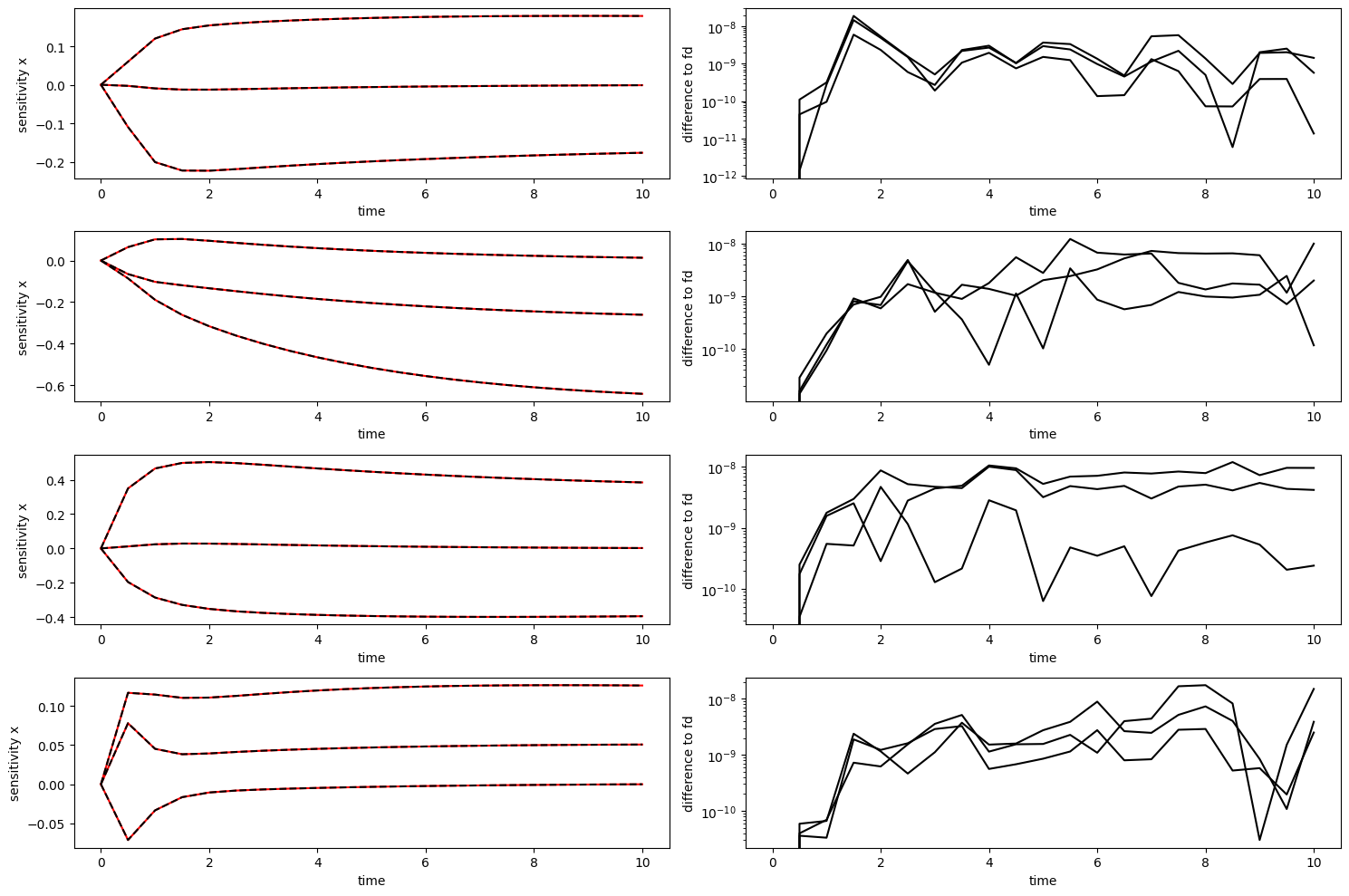
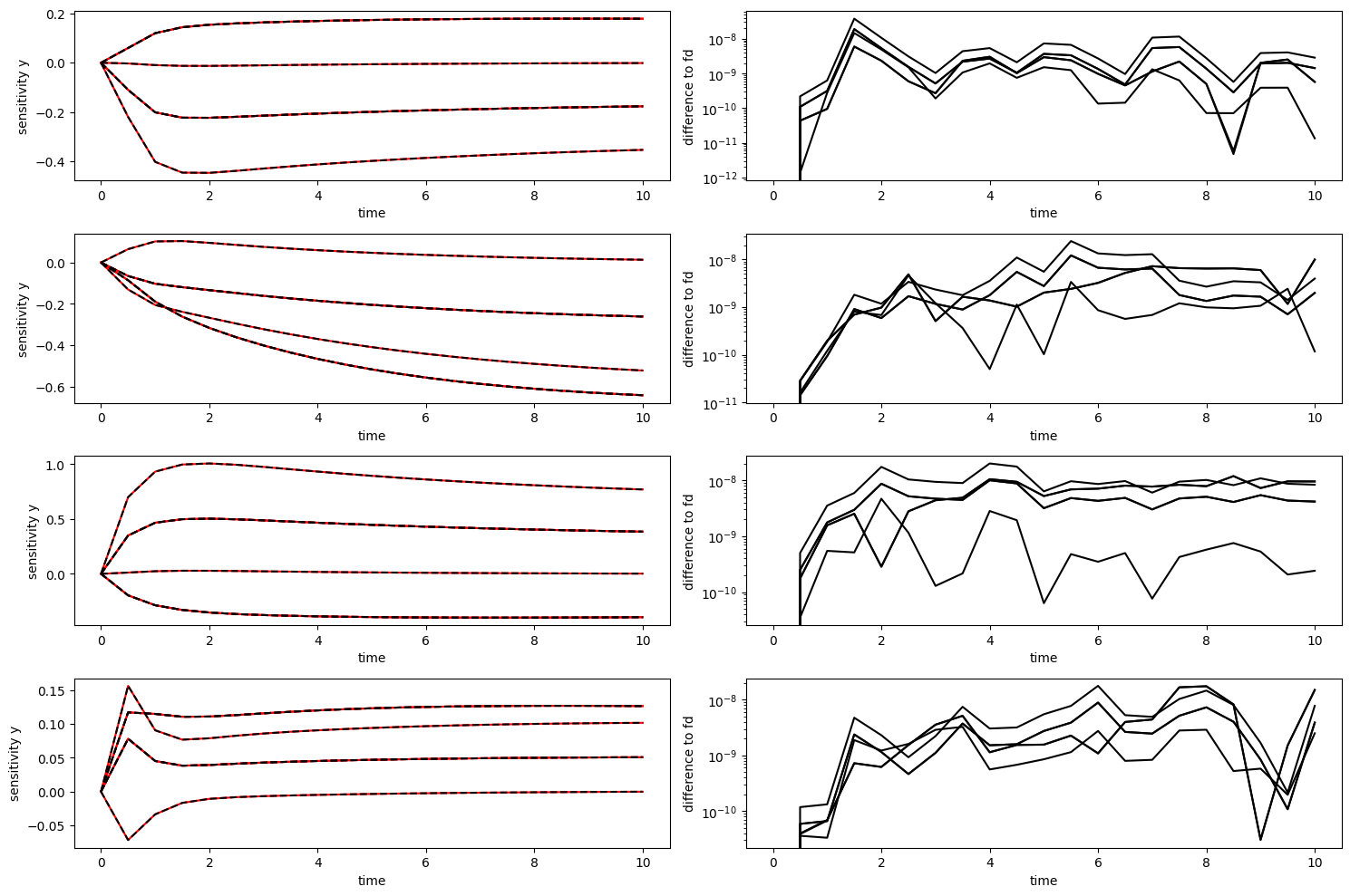
def plot_sensitivities(symbol, eps):
fig, axes = plt.subplots(4, 2, figsize=(15, 10))
for ip in range(4):
fd_approx = fd(model.getParameters(), ip, eps, symbol=symbol)
axes[ip, 0].plot(
edata.getTimepoints(), rdata[f"s{symbol}"][:, ip, :], "r-"
)
axes[ip, 0].plot(edata.getTimepoints(), fd_approx, "k--")
axes[ip, 0].set_ylabel(f"sensitivity {symbol}")
axes[ip, 0].set_xlabel("time")
axes[ip, 1].plot(
edata.getTimepoints(),
np.abs(rdata[f"s{symbol}"][:, ip, :] - fd_approx),
"k-",
)
axes[ip, 1].set_ylabel("difference to fd")
axes[ip, 1].set_xlabel("time")
axes[ip, 1].set_yscale("log")
plt.tight_layout()
plt.show()
[22]:
plot_sensitivities("x", eps)
[23]:
plot_sensitivities("y", eps)
Export as DataFrame
Experimental data and simulation results can both be exported as pandas Dataframe to allow for an easier inspection of numeric values
[24]:
# run the simulation
rdata = amici.runAmiciSimulation(model, solver, edata)
[25]:
# look at the ExpData as DataFrame
df = amici.getDataObservablesAsDataFrame(model, [edata])
df
[25]:
| condition_id | time | datatype | t_presim | k0 | k0_preeq | k0_presim | p1 | p2 | p3 | ... | observable_x3 | observable_x1_scaled | observable_x2_offsetted | observable_x1withsigma | observable_x1_std | observable_x2_std | observable_x3_std | observable_x1_scaled_std | observable_x2_offsetted_std | observable_x1withsigma_std | |
|---|---|---|---|---|---|---|---|---|---|---|---|---|---|---|---|---|---|---|---|---|---|
| 0 | 0.0 | data | 0.0 | 1.0 | NaN | NaN | 1.0 | 0.5 | 0.4 | ... | 0.748067 | 1.007914 | 2.309249 | 0.154751 | 1.0 | 1.0 | 1.0 | 1.0 | 1.0 | NaN | |
| 1 | 0.5 | data | 0.0 | 1.0 | NaN | NaN | 1.0 | 0.5 | 0.4 | ... | 0.140771 | 1.253524 | 4.154876 | 0.613463 | 1.0 | 1.0 | 1.0 | 1.0 | 1.0 | NaN | |
| 2 | 1.0 | data | 0.0 | 1.0 | NaN | NaN | 1.0 | 0.5 | 0.4 | ... | 0.854016 | 1.304569 | 5.426770 | 0.815029 | 1.0 | 1.0 | 1.0 | 1.0 | 1.0 | NaN | |
| 3 | 1.5 | data | 0.0 | 1.0 | NaN | NaN | 1.0 | 0.5 | 0.4 | ... | 0.798610 | -0.397850 | 4.978048 | 1.039835 | 1.0 | 1.0 | 1.0 | 1.0 | 1.0 | NaN | |
| 4 | 2.0 | data | 0.0 | 1.0 | NaN | NaN | 1.0 | 0.5 | 0.4 | ... | -1.440773 | 1.645340 | 4.466585 | 1.012748 | 1.0 | 1.0 | 1.0 | 1.0 | 1.0 | NaN | |
| 5 | 2.5 | data | 0.0 | 1.0 | NaN | NaN | 1.0 | 0.5 | 0.4 | ... | 0.052493 | 2.299055 | 3.632033 | 0.021075 | 1.0 | 1.0 | 1.0 | 1.0 | 1.0 | NaN | |
| 6 | 3.0 | data | 0.0 | 1.0 | NaN | NaN | 1.0 | 0.5 | 0.4 | ... | -1.181170 | 0.673042 | 2.721144 | -0.551402 | 1.0 | 1.0 | 1.0 | 1.0 | 1.0 | NaN | |
| 7 | 3.5 | data | 0.0 | 1.0 | NaN | NaN | 1.0 | 0.5 | 0.4 | ... | 0.273358 | 0.525429 | 3.228554 | 0.841438 | 1.0 | 1.0 | 1.0 | 1.0 | 1.0 | NaN | |
| 8 | 4.0 | data | 0.0 | 1.0 | NaN | NaN | 1.0 | 0.5 | 0.4 | ... | 0.527164 | 1.084840 | 3.590065 | 0.977294 | 1.0 | 1.0 | 1.0 | 1.0 | 1.0 | NaN | |
| 9 | 4.5 | data | 0.0 | 1.0 | NaN | NaN | 1.0 | 0.5 | 0.4 | ... | -1.824907 | 1.356481 | 3.000814 | -1.349610 | 1.0 | 1.0 | 1.0 | 1.0 | 1.0 | NaN | |
| 10 | 5.0 | data | 0.0 | 1.0 | NaN | NaN | 1.0 | 0.5 | 0.4 | ... | 1.039955 | 0.007264 | 5.976927 | -0.522949 | 1.0 | 1.0 | 1.0 | 1.0 | 1.0 | NaN | |
| 11 | 5.5 | data | 0.0 | 1.0 | NaN | NaN | 1.0 | 0.5 | 0.4 | ... | 1.177102 | 1.750903 | 2.471250 | 0.324348 | 1.0 | 1.0 | 1.0 | 1.0 | 1.0 | NaN | |
| 12 | 6.0 | data | 0.0 | 1.0 | NaN | NaN | 1.0 | 0.5 | 0.4 | ... | -0.329617 | -0.739410 | 2.814184 | -0.612429 | 1.0 | 1.0 | 1.0 | 1.0 | 1.0 | NaN | |
| 13 | 6.5 | data | 0.0 | 1.0 | NaN | NaN | 1.0 | 0.5 | 0.4 | ... | -1.344943 | 0.577052 | 2.142942 | 0.096346 | 1.0 | 1.0 | 1.0 | 1.0 | 1.0 | NaN | |
| 14 | 7.0 | data | 0.0 | 1.0 | NaN | NaN | 1.0 | 0.5 | 0.4 | ... | 0.595326 | 0.317392 | 2.010193 | 0.680455 | 1.0 | 1.0 | 1.0 | 1.0 | 1.0 | NaN | |
| 15 | 7.5 | data | 0.0 | 1.0 | NaN | NaN | 1.0 | 0.5 | 0.4 | ... | -0.210457 | 0.059661 | 4.261035 | 1.248413 | 1.0 | 1.0 | 1.0 | 1.0 | 1.0 | NaN | |
| 16 | 8.0 | data | 0.0 | 1.0 | NaN | NaN | 1.0 | 0.5 | 0.4 | ... | -0.442286 | 0.167900 | 3.840273 | 0.717203 | 1.0 | 1.0 | 1.0 | 1.0 | 1.0 | NaN | |
| 17 | 8.5 | data | 0.0 | 1.0 | NaN | NaN | 1.0 | 0.5 | 0.4 | ... | -1.356966 | 2.866951 | 4.052386 | -0.503312 | 1.0 | 1.0 | 1.0 | 1.0 | 1.0 | NaN | |
| 18 | 9.0 | data | 0.0 | 1.0 | NaN | NaN | 1.0 | 0.5 | 0.4 | ... | 0.742708 | 1.079470 | 3.301345 | 0.441377 | 1.0 | 1.0 | 1.0 | 1.0 | 1.0 | NaN | |
| 19 | 9.5 | data | 0.0 | 1.0 | NaN | NaN | 1.0 | 0.5 | 0.4 | ... | -0.145592 | 2.140457 | 5.327872 | 1.897734 | 1.0 | 1.0 | 1.0 | 1.0 | 1.0 | NaN | |
| 20 | 10.0 | data | 0.0 | 1.0 | NaN | NaN | 1.0 | 0.5 | 0.4 | ... | 0.788025 | 1.936927 | 3.323307 | 0.811810 | 1.0 | 1.0 | 1.0 | 1.0 | 1.0 | NaN |
21 rows × 35 columns
[26]:
# from the exported dataframe, we can actually reconstruct a copy of the ExpData instance
reconstructed_edata = amici.getEdataFromDataFrame(model, df)
[27]:
# look at the States in rdata as DataFrame
amici.getResidualsAsDataFrame(model, [edata], [rdata])
[27]:
| condition_id | time | t_presim | k0 | k0_preeq | k0_presim | p1 | p2 | p3 | p4 | ... | p5_scale | scale_scale | offset_scale | sigma_scale | observable_x1 | observable_x2 | observable_x3 | observable_x1_scaled | observable_x2_offsetted | observable_x1withsigma | |
|---|---|---|---|---|---|---|---|---|---|---|---|---|---|---|---|---|---|---|---|---|---|
| 0 | NaN | 0.0 | 0.0 | 1.0 | NaN | NaN | NaN | NaN | NaN | NaN | ... | NaN | NaN | NaN | NaN | 0.190095 | 0.237893 | 0.048067 | 0.807914 | 1.090751 | 0.547510 |
| 1 | NaN | 0.5 | 0.0 | 1.0 | NaN | NaN | NaN | NaN | NaN | NaN | ... | NaN | NaN | NaN | NaN | 0.590463 | 1.168501 | 0.050720 | 0.174789 | 0.470197 | 0.740954 |
| 2 | NaN | 1.0 | 0.0 | 1.0 | NaN | NaN | NaN | NaN | NaN | NaN | ... | NaN | NaN | NaN | NaN | 0.135730 | 0.213488 | 0.757592 | 0.144425 | 1.693483 | 2.349562 |
| 3 | NaN | 1.5 | 0.0 | 1.0 | NaN | NaN | NaN | NaN | NaN | NaN | ... | NaN | NaN | NaN | NaN | 0.425662 | 0.939276 | 0.722534 | 1.538649 | 1.247396 | 4.694355 |
| 4 | NaN | 2.0 | 0.0 | 1.0 | NaN | NaN | NaN | NaN | NaN | NaN | ... | NaN | NaN | NaN | NaN | 0.896601 | 1.460782 | 1.510467 | 0.524270 | 0.750748 | 4.522132 |
| 5 | NaN | 2.5 | 0.0 | 1.0 | NaN | NaN | NaN | NaN | NaN | NaN | ... | NaN | NaN | NaN | NaN | 0.550563 | 0.643982 | 0.013809 | 1.192943 | 0.066718 | 5.319805 |
| 6 | NaN | 3.0 | 0.0 | 1.0 | NaN | NaN | NaN | NaN | NaN | NaN | ... | NaN | NaN | NaN | NaN | 0.664331 | 1.071027 | 1.244903 | 0.420700 | 0.960818 | 10.982727 |
| 7 | NaN | 3.5 | 0.0 | 1.0 | NaN | NaN | NaN | NaN | NaN | NaN | ... | NaN | NaN | NaN | NaN | 1.026232 | 0.319423 | 0.211851 | 0.557291 | 0.437555 | 3.000780 |
| 8 | NaN | 4.0 | 0.0 | 1.0 | NaN | NaN | NaN | NaN | NaN | NaN | ... | NaN | NaN | NaN | NaN | 0.200470 | 0.347285 | 0.467670 | 0.012280 | 0.061237 | 4.410133 |
| 9 | NaN | 4.5 | 0.0 | 1.0 | NaN | NaN | NaN | NaN | NaN | NaN | ... | NaN | NaN | NaN | NaN | 0.310119 | 0.348891 | 1.882560 | 0.293404 | 0.636701 | 18.811478 |
| 10 | NaN | 5.0 | 0.0 | 1.0 | NaN | NaN | NaN | NaN | NaN | NaN | ... | NaN | NaN | NaN | NaN | 1.816659 | 0.926495 | 0.983995 | 1.046918 | 2.352246 | 10.500404 |
| 11 | NaN | 5.5 | 0.0 | 1.0 | NaN | NaN | NaN | NaN | NaN | NaN | ... | NaN | NaN | NaN | NaN | 0.055203 | 1.063313 | 1.122702 | 0.705074 | 1.141483 | 1.985669 |
| 12 | NaN | 6.0 | 0.0 | 1.0 | NaN | NaN | NaN | NaN | NaN | NaN | ... | NaN | NaN | NaN | NaN | 0.061181 | 1.402647 | 0.382576 | 1.777388 | 0.787419 | 11.314185 |
| 13 | NaN | 6.5 | 0.0 | 1.0 | NaN | NaN | NaN | NaN | NaN | NaN | ... | NaN | NaN | NaN | NaN | 0.417778 | 0.929904 | 1.396572 | 0.453546 | 1.448287 | 4.189535 |
| 14 | NaN | 7.0 | 0.0 | 1.0 | NaN | NaN | NaN | NaN | NaN | NaN | ... | NaN | NaN | NaN | NaN | 1.066944 | 0.900330 | 0.544927 | 0.706268 | 1.571362 | 1.686251 |
| 15 | NaN | 7.5 | 0.0 | 1.0 | NaN | NaN | NaN | NaN | NaN | NaN | ... | NaN | NaN | NaN | NaN | 1.369254 | 2.216649 | 0.259716 | 0.957475 | 0.688506 | 7.398453 |
| 16 | NaN | 8.0 | 0.0 | 1.0 | NaN | NaN | NaN | NaN | NaN | NaN | ... | NaN | NaN | NaN | NaN | 0.775327 | 0.796024 | 0.490490 | 0.843100 | 0.276169 | 2.117029 |
| 17 | NaN | 8.5 | 0.0 | 1.0 | NaN | NaN | NaN | NaN | NaN | NaN | ... | NaN | NaN | NaN | NaN | 0.370443 | 1.094272 | 1.404190 | 1.861721 | 0.496152 | 10.059277 |
| 18 | NaN | 9.0 | 0.0 | 1.0 | NaN | NaN | NaN | NaN | NaN | NaN | ... | NaN | NaN | NaN | NaN | 1.361279 | 0.983417 | 0.696393 | 0.079666 | 0.247536 | 0.585248 |
| 19 | NaN | 9.5 | 0.0 | 1.0 | NaN | NaN | NaN | NaN | NaN | NaN | ... | NaN | NaN | NaN | NaN | 0.310327 | 1.076068 | 0.191062 | 1.145757 | 1.785864 | 14.003846 |
| 20 | NaN | 10.0 | 0.0 | 1.0 | NaN | NaN | NaN | NaN | NaN | NaN | ... | NaN | NaN | NaN | NaN | 1.026195 | 1.781992 | 0.743340 | 0.947029 | 0.212274 | 3.168605 |
21 rows × 28 columns
[28]:
# look at the Observables in rdata as DataFrame
amici.getSimulationObservablesAsDataFrame(model, [edata], [rdata])
[28]:
| condition_id | time | datatype | t_presim | k0 | k0_preeq | k0_presim | p1 | p2 | p3 | ... | observable_x3 | observable_x1_scaled | observable_x2_offsetted | observable_x1withsigma | observable_x1_std | observable_x2_std | observable_x3_std | observable_x1_scaled_std | observable_x2_offsetted_std | observable_x1withsigma_std | |
|---|---|---|---|---|---|---|---|---|---|---|---|---|---|---|---|---|---|---|---|---|---|
| 0 | 0.0 | simulation | 0.0 | 1.0 | NaN | NaN | 1.0 | 0.5 | 0.4 | ... | 0.700000 | 0.200000 | 3.400000 | 0.100000 | 1.0 | 1.0 | 1.0 | 1.0 | 1.0 | 0.1 | |
| 1 | 0.5 | simulation | 0.0 | 1.0 | NaN | NaN | 1.0 | 0.5 | 0.4 | ... | 0.191491 | 1.078734 | 3.684679 | 0.539367 | 1.0 | 1.0 | 1.0 | 1.0 | 1.0 | 0.1 | |
| 2 | 1.0 | simulation | 0.0 | 1.0 | NaN | NaN | 1.0 | 0.5 | 0.4 | ... | 0.096424 | 1.160145 | 3.733287 | 0.580072 | 1.0 | 1.0 | 1.0 | 1.0 | 1.0 | 0.1 | |
| 3 | 1.5 | simulation | 0.0 | 1.0 | NaN | NaN | 1.0 | 0.5 | 0.4 | ... | 0.076076 | 1.140799 | 3.730652 | 0.570399 | 1.0 | 1.0 | 1.0 | 1.0 | 1.0 | 0.1 | |
| 4 | 2.0 | simulation | 0.0 | 1.0 | NaN | NaN | 1.0 | 0.5 | 0.4 | ... | 0.069694 | 1.121069 | 3.715836 | 0.560535 | 1.0 | 1.0 | 1.0 | 1.0 | 1.0 | 0.1 | |
| 5 | 2.5 | simulation | 0.0 | 1.0 | NaN | NaN | 1.0 | 0.5 | 0.4 | ... | 0.066301 | 1.106112 | 3.698751 | 0.553056 | 1.0 | 1.0 | 1.0 | 1.0 | 1.0 | 0.1 | |
| 6 | 3.0 | simulation | 0.0 | 1.0 | NaN | NaN | 1.0 | 0.5 | 0.4 | ... | 0.063733 | 1.093741 | 3.681963 | 0.546871 | 1.0 | 1.0 | 1.0 | 1.0 | 1.0 | 0.1 | |
| 7 | 3.5 | simulation | 0.0 | 1.0 | NaN | NaN | 1.0 | 0.5 | 0.4 | ... | 0.061506 | 1.082720 | 3.666109 | 0.541360 | 1.0 | 1.0 | 1.0 | 1.0 | 1.0 | 0.1 | |
| 8 | 4.0 | simulation | 0.0 | 1.0 | NaN | NaN | 1.0 | 0.5 | 0.4 | ... | 0.059495 | 1.072561 | 3.651302 | 0.536280 | 1.0 | 1.0 | 1.0 | 1.0 | 1.0 | 0.1 | |
| 9 | 4.5 | simulation | 0.0 | 1.0 | NaN | NaN | 1.0 | 0.5 | 0.4 | ... | 0.057653 | 1.063076 | 3.637515 | 0.531538 | 1.0 | 1.0 | 1.0 | 1.0 | 1.0 | 0.1 | |
| 10 | 5.0 | simulation | 0.0 | 1.0 | NaN | NaN | 1.0 | 0.5 | 0.4 | ... | 0.055960 | 1.054183 | 3.624681 | 0.527091 | 1.0 | 1.0 | 1.0 | 1.0 | 1.0 | 0.1 | |
| 11 | 5.5 | simulation | 0.0 | 1.0 | NaN | NaN | 1.0 | 0.5 | 0.4 | ... | 0.054400 | 1.045829 | 3.612733 | 0.522914 | 1.0 | 1.0 | 1.0 | 1.0 | 1.0 | 0.1 | |
| 12 | 6.0 | simulation | 0.0 | 1.0 | NaN | NaN | 1.0 | 0.5 | 0.4 | ... | 0.052960 | 1.037978 | 3.601603 | 0.518989 | 1.0 | 1.0 | 1.0 | 1.0 | 1.0 | 0.1 | |
| 13 | 6.5 | simulation | 0.0 | 1.0 | NaN | NaN | 1.0 | 0.5 | 0.4 | ... | 0.051629 | 1.030598 | 3.591229 | 0.515299 | 1.0 | 1.0 | 1.0 | 1.0 | 1.0 | 0.1 | |
| 14 | 7.0 | simulation | 0.0 | 1.0 | NaN | NaN | 1.0 | 0.5 | 0.4 | ... | 0.050399 | 1.023660 | 3.581555 | 0.511830 | 1.0 | 1.0 | 1.0 | 1.0 | 1.0 | 0.1 | |
| 15 | 7.5 | simulation | 0.0 | 1.0 | NaN | NaN | 1.0 | 0.5 | 0.4 | ... | 0.049259 | 1.017136 | 3.572529 | 0.508568 | 1.0 | 1.0 | 1.0 | 1.0 | 1.0 | 0.1 | |
| 16 | 8.0 | simulation | 0.0 | 1.0 | NaN | NaN | 1.0 | 0.5 | 0.4 | ... | 0.048203 | 1.011000 | 3.564103 | 0.505500 | 1.0 | 1.0 | 1.0 | 1.0 | 1.0 | 0.1 | |
| 17 | 8.5 | simulation | 0.0 | 1.0 | NaN | NaN | 1.0 | 0.5 | 0.4 | ... | 0.047224 | 1.005231 | 3.556234 | 0.502615 | 1.0 | 1.0 | 1.0 | 1.0 | 1.0 | 0.1 | |
| 18 | 9.0 | simulation | 0.0 | 1.0 | NaN | NaN | 1.0 | 0.5 | 0.4 | ... | 0.046315 | 0.999804 | 3.548881 | 0.499902 | 1.0 | 1.0 | 1.0 | 1.0 | 1.0 | 0.1 | |
| 19 | 9.5 | simulation | 0.0 | 1.0 | NaN | NaN | 1.0 | 0.5 | 0.4 | ... | 0.045471 | 0.994700 | 3.542008 | 0.497350 | 1.0 | 1.0 | 1.0 | 1.0 | 1.0 | 0.1 | |
| 20 | 10.0 | simulation | 0.0 | 1.0 | NaN | NaN | 1.0 | 0.5 | 0.4 | ... | 0.044686 | 0.989898 | 3.535581 | 0.494949 | 1.0 | 1.0 | 1.0 | 1.0 | 1.0 | 0.1 |
21 rows × 35 columns
[29]:
# look at the States in rdata as DataFrame
amici.getSimulationStatesAsDataFrame(model, [edata], [rdata])
[29]:
| condition_id | time | t_presim | k0 | k0_preeq | k0_presim | p1 | p2 | p3 | p4 | ... | p2_scale | p3_scale | p4_scale | p5_scale | scale_scale | offset_scale | sigma_scale | x1 | x2 | x3 | |
|---|---|---|---|---|---|---|---|---|---|---|---|---|---|---|---|---|---|---|---|---|---|
| 0 | 0.0 | 0.0 | 1.0 | NaN | NaN | 1.0 | 0.5 | 0.4 | 2.0 | ... | 0 | 0 | 0 | 0 | 0 | 0 | 0 | 0.100000 | 0.400000 | 0.700000 | |
| 1 | 0.5 | 0.0 | 1.0 | NaN | NaN | 1.0 | 0.5 | 0.4 | 2.0 | ... | 0 | 0 | 0 | 0 | 0 | 0 | 0 | 0.539367 | 0.684679 | 0.191491 | |
| 2 | 1.0 | 0.0 | 1.0 | NaN | NaN | 1.0 | 0.5 | 0.4 | 2.0 | ... | 0 | 0 | 0 | 0 | 0 | 0 | 0 | 0.580072 | 0.733287 | 0.096424 | |
| 3 | 1.5 | 0.0 | 1.0 | NaN | NaN | 1.0 | 0.5 | 0.4 | 2.0 | ... | 0 | 0 | 0 | 0 | 0 | 0 | 0 | 0.570399 | 0.730652 | 0.076076 | |
| 4 | 2.0 | 0.0 | 1.0 | NaN | NaN | 1.0 | 0.5 | 0.4 | 2.0 | ... | 0 | 0 | 0 | 0 | 0 | 0 | 0 | 0.560535 | 0.715836 | 0.069694 | |
| 5 | 2.5 | 0.0 | 1.0 | NaN | NaN | 1.0 | 0.5 | 0.4 | 2.0 | ... | 0 | 0 | 0 | 0 | 0 | 0 | 0 | 0.553056 | 0.698751 | 0.066301 | |
| 6 | 3.0 | 0.0 | 1.0 | NaN | NaN | 1.0 | 0.5 | 0.4 | 2.0 | ... | 0 | 0 | 0 | 0 | 0 | 0 | 0 | 0.546871 | 0.681963 | 0.063733 | |
| 7 | 3.5 | 0.0 | 1.0 | NaN | NaN | 1.0 | 0.5 | 0.4 | 2.0 | ... | 0 | 0 | 0 | 0 | 0 | 0 | 0 | 0.541360 | 0.666109 | 0.061506 | |
| 8 | 4.0 | 0.0 | 1.0 | NaN | NaN | 1.0 | 0.5 | 0.4 | 2.0 | ... | 0 | 0 | 0 | 0 | 0 | 0 | 0 | 0.536280 | 0.651302 | 0.059495 | |
| 9 | 4.5 | 0.0 | 1.0 | NaN | NaN | 1.0 | 0.5 | 0.4 | 2.0 | ... | 0 | 0 | 0 | 0 | 0 | 0 | 0 | 0.531538 | 0.637515 | 0.057653 | |
| 10 | 5.0 | 0.0 | 1.0 | NaN | NaN | 1.0 | 0.5 | 0.4 | 2.0 | ... | 0 | 0 | 0 | 0 | 0 | 0 | 0 | 0.527091 | 0.624681 | 0.055960 | |
| 11 | 5.5 | 0.0 | 1.0 | NaN | NaN | 1.0 | 0.5 | 0.4 | 2.0 | ... | 0 | 0 | 0 | 0 | 0 | 0 | 0 | 0.522914 | 0.612733 | 0.054400 | |
| 12 | 6.0 | 0.0 | 1.0 | NaN | NaN | 1.0 | 0.5 | 0.4 | 2.0 | ... | 0 | 0 | 0 | 0 | 0 | 0 | 0 | 0.518989 | 0.601603 | 0.052960 | |
| 13 | 6.5 | 0.0 | 1.0 | NaN | NaN | 1.0 | 0.5 | 0.4 | 2.0 | ... | 0 | 0 | 0 | 0 | 0 | 0 | 0 | 0.515299 | 0.591229 | 0.051629 | |
| 14 | 7.0 | 0.0 | 1.0 | NaN | NaN | 1.0 | 0.5 | 0.4 | 2.0 | ... | 0 | 0 | 0 | 0 | 0 | 0 | 0 | 0.511830 | 0.581555 | 0.050399 | |
| 15 | 7.5 | 0.0 | 1.0 | NaN | NaN | 1.0 | 0.5 | 0.4 | 2.0 | ... | 0 | 0 | 0 | 0 | 0 | 0 | 0 | 0.508568 | 0.572529 | 0.049259 | |
| 16 | 8.0 | 0.0 | 1.0 | NaN | NaN | 1.0 | 0.5 | 0.4 | 2.0 | ... | 0 | 0 | 0 | 0 | 0 | 0 | 0 | 0.505500 | 0.564103 | 0.048203 | |
| 17 | 8.5 | 0.0 | 1.0 | NaN | NaN | 1.0 | 0.5 | 0.4 | 2.0 | ... | 0 | 0 | 0 | 0 | 0 | 0 | 0 | 0.502615 | 0.556234 | 0.047224 | |
| 18 | 9.0 | 0.0 | 1.0 | NaN | NaN | 1.0 | 0.5 | 0.4 | 2.0 | ... | 0 | 0 | 0 | 0 | 0 | 0 | 0 | 0.499902 | 0.548881 | 0.046315 | |
| 19 | 9.5 | 0.0 | 1.0 | NaN | NaN | 1.0 | 0.5 | 0.4 | 2.0 | ... | 0 | 0 | 0 | 0 | 0 | 0 | 0 | 0.497350 | 0.542008 | 0.045471 | |
| 20 | 10.0 | 0.0 | 1.0 | NaN | NaN | 1.0 | 0.5 | 0.4 | 2.0 | ... | 0 | 0 | 0 | 0 | 0 | 0 | 0 | 0.494949 | 0.535581 | 0.044686 |
21 rows × 25 columns