Spline implementation of JAK2-STAT5 signaling pathway

In this notebook a practical example of the usage of AMICI spline functionalities is shown. The model under consideration is the JAK2-STAT5 signaling pathway (Swameye et al., 2003), in which the dynamics of the system depend on a measured input function (the quantity pEpoR in the model).

Following the approach of (Schelker et al., 2012), a continuous approximation of this input function is estimated together with the other parameters. As in the original paper, we will use a spline with logarithmic parameterization in order to enforce the positivity constraint.

The model of the signaling pathway will be implemented in SBML using AMICI’s spline annotations, experimental data integrated using the PEtab format and parameter estimation will be carried out using the pyPESTO library.

%pip install pypesto

%pip install fides

import copy
import logging
import os

import libsbml
import numpy as np
import pandas as pd
import petab
import pypesto.petab
import sympy as sp
from matplotlib import pyplot as plt

import amici

# Number of multi-starts for MAP estimation
n_starts = 150
# n_starts = 0 # when loading results

# Set default pypesto engine/optimizer
pypesto_optimizer = pypesto.optimize.FidesOptimizer(verbose=logging.WARNING)
pypesto_engine = pypesto.engine.MultiProcessEngine()

# If running as a GitHub action, just do the minimal amount of work required to check whether the code is working
if os.getenv("GITHUB_ACTIONS") is not None:
    n_starts = 25
    pypesto_optimizer = pypesto.optimize.FidesOptimizer(
        verbose=logging.WARNING, options=dict(maxiter=10)
    )
    pypesto_engine = pypesto.engine.MultiProcessEngine()

# A dictionary to store different approaches for a final comparison
all_results = {}

Spline approximation with few nodes, using finite differences for the derivatives

As a first attempt, we fix a small amount of nodes, create new parameters for the values of the splines at the nodes and let AMICI compute the derivative at the nodes by using finite differences.

Creating the PEtab model

# Problem name
name = "Swameye_PNAS2003_5nodes_FD"

First, we create a spline to represent the input function pEpoR, parametrized by its values at the nodes. Since the value of the input function reaches its steady state by the end of the experiment, we extrapolate constantly after that (useful if we need to simulate the model after the last spline node).

# Create spline for pEpoR
nodes = [0, 5, 10, 20, 60]
values_at_nodes = [
    sp.Symbol(f"pEpoR_t{str(t).replace('.', '_dot_')}") for t in nodes
]  # new parameter symbols for spline values
spline = amici.splines.CubicHermiteSpline(
    sbml_id="pEpoR",  # matches name of species in SBML model
    evaluate_at=amici.sbml_utils.amici_time_symbol,  # the spline is evaluated at the current time
    nodes=nodes,
    values_at_nodes=values_at_nodes,  # values at the nodes (in linear scale)
    extrapolate=(None, "constant"),  # because steady state is reached
    bc="auto",  # automatically determined from extrapolate (bc at right end will be 'zero_derivative')
    logarithmic_parametrization=True,
)

We can then add the spline to a skeleton SBML model based on the d2d implementation by (Schelker et al., 2012). The skeleton SBML model defines a species pEpoR which interacts with the other species, but has no reactions or rate rules of its own. The code below creates an assignment rule for pEpoR using the spline formula, completing the model. The parameters pEpoR_t* are automatically added to the SBML model too (using nominal values of 0.1 and declaring them to be constant).

# Add spline formula to SBML model
sbml_doc = libsbml.SBMLReader().readSBML(
    os.path.join("Swameye_PNAS2003", "swameye2003_model.xml")
)
sbml_model = sbml_doc.getModel()
spline.add_to_sbml_model(
    sbml_model, auto_add=True, y_nominal=0.1, y_constant=True
)

A skeleton PEtab problem is provided, containing parameter bounds, observable definitions and experimental data. Of particular relevance is the noise model used for the measurements of pEpoR, normal additive noise with standard deviation equal to 0.0274 + 0.1 * pEpoR; this is the same choice used in (Schelker et al., 2012), where it was estimated from experimental replicates.

However, the parameters associated to the spline are to be added too. The code below defines parameter bounds for them according to the PEtab format and then creates a full PEtab problem integrating them together with the edited SBML file. The condition, measurement and observable PEtab tables do not require additional modification and can be used as they are.

# Extra parameters associated to the spline
spline_parameters_df = pd.DataFrame(
    dict(
        parameterScale="log",
        lowerBound=0.001,
        upperBound=10,
        nominalValue=0.1,
        estimate=1,
    ),
    index=pd.Series(list(map(str, values_at_nodes)), name="parameterId"),
)

# Create PEtab problem
petab_problem = petab.Problem(
    sbml_model,
    condition_df=petab.conditions.get_condition_df(
        os.path.join("Swameye_PNAS2003", "swameye2003_conditions.tsv")
    ),
    measurement_df=petab.measurements.get_measurement_df(
        os.path.join("Swameye_PNAS2003", "swameye2003_measurements.tsv")
    ),
    parameter_df=petab.core.concat_tables(
        [
            os.path.join("Swameye_PNAS2003", "swameye2003_parameters.tsv"),
            spline_parameters_df,
        ],
        petab.parameters.get_parameter_df,
    ),
    observable_df=petab.observables.get_observable_df(
        os.path.join("Swameye_PNAS2003", "swameye2003_observables.tsv")
    ),
)

The resulting PEtab problem can be checked for errors and exported to disk if needed.

# Check whether PEtab model is valid
assert not petab.lint_problem(petab_problem)

# Save PEtab problem to disk
# import shutil
# shutil.rmtree(name, ignore_errors=True)
# os.mkdir(name)
# petab_problem.to_files_generic(prefix_path=name)

Creating the pyPESTO problem

We can now create a pyPESTO problem directly from the PEtab problem. Due to technical limitations in AMICI, currently the PEtab problem has to be “flattened” before it can be simulated from, but such operation is merely syntactical and thus does not change the essence of the model.

# Problem must be "flattened" to be used with AMICI
petab.core.flatten_timepoint_specific_output_overrides(petab_problem)

# Check whether simulation from the PEtab problem works
# import amici.petab_simulate
# simulator = amici.petab_simulate.PetabSimulator(petab_problem)
# simulator.simulate(noise=False)

# Import PEtab problem into pyPESTO
pypesto_problem = pypesto.petab.PetabImporter(
    petab_problem, model_name=name
).create_problem()

# Increase maximum number of steps for AMICI
pypesto_problem.objective.amici_solver.setMaxSteps(10**5)

Maximum Likelihood estimation

Using pyPESTO we can optimize for the parameter vector that maximizes the probability of observing the experimental data (maximum likelihood estimation).

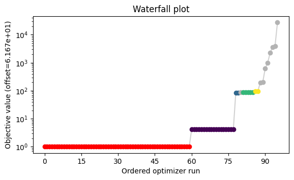
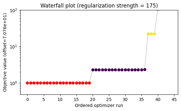
A multistart method with local gradient-based optimization is used and the results of each multistart can be visualized in a waterfall plot.

# Load existing results if available
if os.path.exists(f"{name}.h5"):
    pypesto_result = pypesto.store.read_result(
        f"{name}.h5", problem=pypesto_problem
    )
else:
    pypesto_result = None
# Overwrite
# pypesto_result = None

# Parallel multistart optimization with pyPESTO and FIDES
if n_starts > 0:
    if pypesto_result is None:
        new_ids = [str(i) for i in range(n_starts)]
    else:
        last_id = max(int(i) for i in pypesto_result.optimize_result.id)
        new_ids = [str(i) for i in range(last_id + 1, last_id + n_starts + 1)]
    pypesto_result = pypesto.optimize.minimize(
        pypesto_problem,
        n_starts=n_starts,
        ids=new_ids,
        optimizer=pypesto_optimizer,
        engine=pypesto_engine,
        result=pypesto_result,
    )
    pypesto_result.optimize_result.sort()
    if pypesto_result.optimize_result.x[0] is None:
        raise Exception(
            "All multistarts failed (n_starts is probably too small)! If this error occurred during CI, just run the workflow again."
        )

# Save results to disk
# pypesto.store.write_result(pypesto_result, f'{name}.h5', overwrite=True)

# Print result table
# pypesto_result.optimize_result.as_dataframe()

# Visualize the results of the multistarts
pypesto.visualize.waterfall(pypesto_result, size=[6.5, 3.5]);

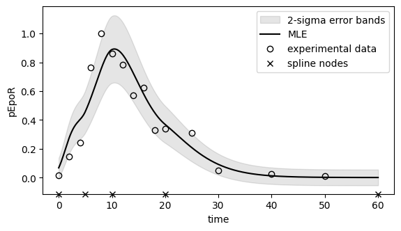
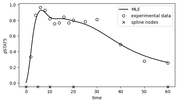
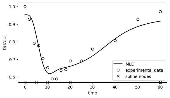
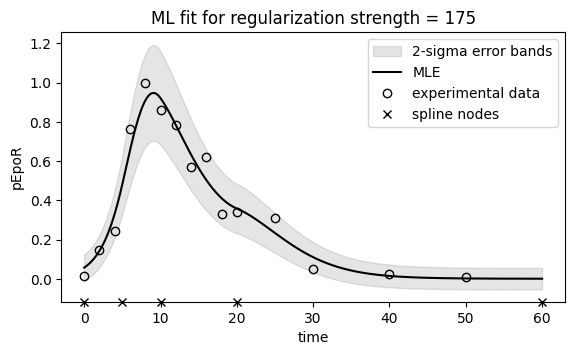
Below the maximum likelihood estimates for pEpoR and the other observables are plotted, together with the experimental measurements.

To assess whether the noise model used in the observable is reasonable, we have also plotted 2-sigma error bands for pEpoR.

# Functions for simulating observables given a parameter vector
def _simulate(x=None, *, problem=None, result=None, N=500, **kwargs):
    if result is None:
        result = pypesto_result
    if problem is None:
        problem = pypesto_problem
    if x is None:
        x = result.optimize_result.x[0]
    if N is None:
        objective = problem.objective
    else:
        objective = problem.objective.set_custom_timepoints(
            timepoints_global=np.linspace(0, 60, N)
        )
    if len(x) != len(problem.x_free_indices):
        x = x[problem.x_free_indices]
    simresult = objective(x, return_dict=True, **kwargs)
    return problem, simresult["rdatas"][0]


def simulate_pEpoR(x=None, **kwargs):
    problem, rdata = _simulate(x, **kwargs)
    assert problem.objective.amici_model.getObservableIds()[0].startswith(
        "pEpoR"
    )
    return rdata["t"], rdata["y"][:, 0]


def simulate_pSTAT5(x=None, **kwargs):
    problem, rdata = _simulate(x, **kwargs)
    assert problem.objective.amici_model.getObservableIds()[1].startswith(
        "pSTAT5"
    )
    return rdata["t"], rdata["y"][:, 1]


def simulate_tSTAT5(x=None, **kwargs):
    problem, rdata = _simulate(x, **kwargs)
    assert problem.objective.amici_model.getObservableIds()[-1].startswith(
        "tSTAT5"
    )
    return rdata["t"], rdata["y"][:, -1]


# Experimental data
df_measurements = petab.measurements.get_measurement_df(
    os.path.join("Swameye_PNAS2003", "swameye2003_measurements.tsv")
)
df_pEpoR = df_measurements[
    df_measurements["observableId"].str.startswith("pEpoR")
]
df_pSTAT5 = df_measurements[
    df_measurements["observableId"].str.startswith("pSTAT5")
]
df_tSTAT5 = df_measurements[
    df_measurements["observableId"].str.startswith("tSTAT5")
]

# Plot ML fit for pEpoR
fig, ax = plt.subplots(figsize=(6.5, 3.5))
t, pEpoR = simulate_pEpoR()
sigma_pEpoR = 0.0274 + 0.1 * pEpoR
ax.fill_between(
    t,
    pEpoR - 2 * sigma_pEpoR,
    pEpoR + 2 * sigma_pEpoR,
    color="black",
    alpha=0.10,
    interpolate=True,
    label="2-sigma error bands",
)
ax.plot(t, pEpoR, color="black", label="MLE")
ax.plot(
    df_pEpoR["time"],
    df_pEpoR["measurement"],
    "o",
    color="black",
    markerfacecolor="none",
    label="experimental data",
)
ylim1 = ax.get_ylim()[0]
ax.plot(
    nodes,
    len(nodes) * [ylim1],
    "x",
    color="black",
    label="spline nodes",
    zorder=10,
    clip_on=False,
)
ax.set_ylim(ylim1, ax.get_ylim()[1])
ax.set_xlabel("time")
ax.set_ylabel("pEpoR")
ax.legend();

# Plot ML fit for pSTAT5
fig, ax = plt.subplots(figsize=(6.5, 3.5))
t, pSTAT5 = simulate_pSTAT5()
ax.plot(t, pSTAT5, color="black", label="MLE")
ax.plot(
    df_pSTAT5["time"],
    df_pSTAT5["measurement"],
    "o",
    color="black",
    markerfacecolor="none",
    label="experimental data",
)
ylim1 = ax.get_ylim()[0]
ax.plot(
    nodes,
    len(nodes) * [ylim1],
    "x",
    color="black",
    label="spline nodes",
    zorder=10,
    clip_on=False,
)
ax.set_ylim(ylim1, ax.get_ylim()[1])
ax.set_xlabel("time")
ax.set_ylabel("pSTAT5")
ax.legend();

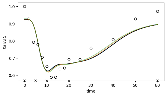
# Plot ML fit for tSTAT5
fig, ax = plt.subplots(figsize=(6.5, 3.5))
t, tSTAT5 = simulate_tSTAT5()
ax.plot(t, tSTAT5, color="black", label="MLE")
ax.plot(
    df_tSTAT5["time"],
    df_tSTAT5["measurement"],
    "o",
    color="black",
    markerfacecolor="none",
    label="experimental data",
)
ylim1 = ax.get_ylim()[0]
ax.plot(
    nodes,
    len(nodes) * [ylim1],
    "x",
    color="black",
    label="spline nodes",
    zorder=10,
    clip_on=False,
)
ax.set_ylim(ylim1, ax.get_ylim()[1])
ax.set_xlabel("time")
ax.set_ylabel("tSTAT5")
ax.legend();

# Store results for later
all_results["5 nodes, FD"] = (pypesto_problem, pypesto_result)

Spline approximation with many nodes, using finite differences for the derivatives

Five nodes is arguably not enough to represent all plausible input choices. Increasing the number of nodes would give the spline more freedom and it can be done with minimal changes to the example above. However, more degrees of freedom mean more chance of overfitting. Thus, following (Schelker et al., 2012), we will add a regularization term consisting in the squared L2 norm of the spline’s curvature, which promotes smoother and less oscillating functions. The value for the regularization strength \(\lambda\) is chosen by comparing the sum of squared normalized residuals with its expected value, which can be computing by assuming it is roughly \(\chi^2\)-distributed.

Creating the PEtab model

# Problem name
name = "Swameye_PNAS2003_15nodes_FD"

# Create spline for pEpoR
nodes = [0, 2.5, 5.0, 7.5, 10.0, 12.5, 15.0, 17.5, 20, 25, 30, 35, 40, 50, 60]
values_at_nodes = [
    sp.Symbol(f"pEpoR_t{str(t).replace('.', '_dot_')}") for t in nodes
]
spline = amici.splines.CubicHermiteSpline(
    sbml_id="pEpoR",
    evaluate_at=amici.sbml_utils.amici_time_symbol,
    nodes=nodes,
    values_at_nodes=values_at_nodes,
    extrapolate=(None, "constant"),
    bc="auto",
    logarithmic_parametrization=True,
)

The regularization term can be easily computed by symbolic manipulation of the spline expression using AMICI and SymPy. Since it is very commonly used, we already provide a function for it in AMICI. Note: we regularize the curvature of the spline, which for positivity-enforcing spline is the logarithm of the function.

In order add the regularization term to the PEtab likelihood, a dummy observable has to be created.

# Compute L2 norm of the curvature of pEpoR
regularization = spline.squared_L2_norm_of_curvature()

# Add a parameter for regularization strength
reg_parameters_df = pd.DataFrame(
    dict(
        parameterScale="log10",
        lowerBound=1e-6,
        upperBound=1e6,
        nominalValue=1.0,
        estimate=0,
    ),
    index=pd.Series(["regularization_strength"], name="parameterId"),
)
# Encode regularization term as an additional observable
reg_observables_df = pd.DataFrame(
    dict(
        observableFormula=f"sqrt({regularization})".replace("**", "^"),
        observableTransformation="lin",
        noiseFormula="1/sqrt(regularization_strength)",
        noiseDistribution="normal",
    ),
    index=pd.Series(["regularization"], name="observableId"),
)
# and correspoding measurement
reg_measurements_df = pd.DataFrame(
    dict(
        observableId="regularization",
        simulationConditionId="condition1",
        measurement=0,
        time=0,
        observableTransformation="lin",
    ),
    index=pd.Series([0]),
)

# Add spline formula to SBML model
sbml_doc = libsbml.SBMLReader().readSBML(
    os.path.join("Swameye_PNAS2003", "swameye2003_model.xml")
)
sbml_model = sbml_doc.getModel()
spline.add_to_sbml_model(
    sbml_model, auto_add=True, y_nominal=0.1, y_constant=True
)

# Extra parameters associated to the spline
spline_parameters_df = pd.DataFrame(
    dict(
        parameterScale="log",
        lowerBound=0.001,
        upperBound=10,
        nominalValue=0.1,
        estimate=1,
    ),
    index=pd.Series(list(map(str, values_at_nodes)), name="parameterId"),
)

# Create PEtab problem
petab_problem = petab.Problem(
    sbml_model,
    condition_df=petab.conditions.get_condition_df(
        os.path.join("Swameye_PNAS2003", "swameye2003_conditions.tsv")
    ),
    measurement_df=petab.core.concat_tables(
        [
            os.path.join("Swameye_PNAS2003", "swameye2003_measurements.tsv"),
            reg_measurements_df,
        ],
        petab.measurements.get_measurement_df,
    ).reset_index(drop=True),
    parameter_df=petab.core.concat_tables(
        [
            os.path.join("Swameye_PNAS2003", "swameye2003_parameters.tsv"),
            spline_parameters_df,
            reg_parameters_df,
        ],
        petab.parameters.get_parameter_df,
    ),
    observable_df=petab.core.concat_tables(
        [
            os.path.join("Swameye_PNAS2003", "swameye2003_observables.tsv"),
            reg_observables_df,
        ],
        petab.observables.get_observable_df,
    ),
)

# Check whether PEtab model is valid
assert not petab.lint_problem(petab_problem)

# Save PEtab problem to disk
# import shutil
# shutil.rmtree(name, ignore_errors=True)
# os.mkdir(name)
# petab_problem.to_files_generic(prefix_path=name)

Creating the pyPESTO problem

# Problem must be "flattened" to be used with AMICI
petab.core.flatten_timepoint_specific_output_overrides(petab_problem)

# Check whether simulation from the PEtab problem works
# import amici.petab_simulate
# simulator = amici.petab_simulate.PetabSimulator(petab_problem)
# simulator.simulate(noise=False)

# Import PEtab problem into pyPESTO
pypesto_problem = pypesto.petab.PetabImporter(
    petab_problem, model_name=name
).create_problem()

Maximum Likelihood estimation

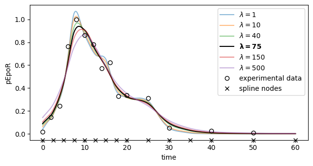
We will optimize the problem for different values of the regularization strength \(\lambda\), then compute the sum of squared normalized residuals for each of the resulting parameter vectors. The one for which such a value is nearest to its expected value of \(15\) (the number of observations from the input function) will be chosen as the final estimate.

# Try different regularization strengths
regstrengths = np.asarray([1, 10, 40, 75, 150, 500])
if os.getenv("GITHUB_ACTIONS") is not None:
    regstrengths = np.asarray([75])
regproblems = {}
regresults = {}

for regstrength in regstrengths:
    # Fix parameter in pypesto problem
    name = f"Swameye_PNAS2003_15nodes_FD_reg{regstrength}"
    pypesto_problem.fix_parameters(
        pypesto_problem.x_names.index("regularization_strength"),
        np.log10(
            regstrength
        ),  # parameter is specified as log10 scale in PEtab
    )
    regproblem = copy.deepcopy(pypesto_problem)

    # Load existing results if available
    if os.path.exists(f"{name}.h5"):
        regresult = pypesto.store.read_result(f"{name}.h5", problem=regproblem)
    else:
        regresult = None
    # Overwrite
    # regresult = None

    # Parallel multistart optimization with pyPESTO and FIDES
    if n_starts > 0:
        if regresult is None:
            new_ids = [str(i) for i in range(n_starts)]
        else:
            last_id = max(int(i) for i in regresult.optimize_result.id)
            new_ids = [
                str(i) for i in range(last_id + 1, last_id + n_starts + 1)
            ]
        regresult = pypesto.optimize.minimize(
            regproblem,
            n_starts=n_starts,
            ids=new_ids,
            optimizer=pypesto_optimizer,
            engine=pypesto_engine,
            result=regresult,
        )
        regresult.optimize_result.sort()
        if regresult.optimize_result.x[0] is None:
            raise Exception(
                "All multistarts failed (n_starts is probably too small)! If this error occurred during CI, just run the workflow again."
            )

    # Save results to disk
    # pypesto.store.write_result(regresult, f'{name}.h5', overwrite=True)

    # Store result
    regproblems[regstrength] = regproblem
    regresults[regstrength] = regresult

# Compute sum of squared normalized residuals
print(f"Target value is {len(df_pEpoR['time'])}")
regstrengths = sorted(regproblems.keys())
stats = []
for regstrength in regstrengths:
    t, pEpoR = simulate_pEpoR(
        N=None,
        problem=regproblems[regstrength],
        result=regresults[regstrength],
    )
    assert np.array_equal(df_pEpoR["time"], t[:-1])
    pEpoR = pEpoR[:-1]
    sigma_pEpoR = 0.0274 + 0.1 * pEpoR
    stat = np.sum(((pEpoR - df_pEpoR["measurement"]) / sigma_pEpoR) ** 2)
    print(f"Regularization strength: {regstrength}. Statistic is {stat}")
    stats.append(stat)
# Select best regularization strength
chosen_regstrength = regstrengths[
    np.abs(np.asarray(stats) - len(df_pEpoR["time"])).argmin()
]

Target value is 15
Regularization strength: 1. Statistic is 6.794369874307712
Regularization strength: 10. Statistic is 8.435094498146606
Regularization strength: 40. Statistic is 11.83872830962955
Regularization strength: 75. Statistic is 15.030926511510327
Regularization strength: 150. Statistic is 19.971139477161476
Regularization strength: 500. Statistic is 32.44623424533765

# Visualize the results of the multistarts for a chosen regularization strength
ax = pypesto.visualize.waterfall(
    regresults[chosen_regstrength], size=[6.5, 3.5]
)
ax.set_title(
    f"Waterfall plot (regularization strength = {chosen_regstrength})"
)
ax.set_ylim(ax.get_ylim()[0], 100);

# Plot ML fit for pEpoR (all regularization strengths)
fig, ax = plt.subplots(figsize=(6.5, 3.5))
for regstrength in sorted(regproblems.keys()):
    t, pEpoR = simulate_pEpoR(
        problem=regproblems[regstrength], result=regresults[regstrength]
    )
    if regstrength == chosen_regstrength:
        kwargs = dict(
            color="black",
            label=f"$\\mathbf{{\\lambda = {regstrength}}}$",
            zorder=2,
        )
    else:
        kwargs = dict(label=f"$\\lambda = {regstrength}$", alpha=0.5)
    ax.plot(t, pEpoR, **kwargs)
ax.plot(
    df_pEpoR["time"],
    df_pEpoR["measurement"],
    "o",
    color="black",
    markerfacecolor="none",
    label="experimental data",
)
ylim1 = ax.get_ylim()[0]
ax.plot(
    nodes,
    len(nodes) * [ylim1],
    "x",
    color="black",
    label="spline nodes",
    zorder=10,
    clip_on=False,
)
ax.set_ylim(ylim1, ax.get_ylim()[1])
ax.set_xlabel("time")
ax.set_ylabel("pEpoR")
ax.set_xlim(-3.0, 63.0)
ax.set_ylim(-0.05299052022388704, 1.126290214024833)
ax.legend()
ax.figure.tight_layout()
# ax.set_ylabel("input function")
# print(f"xlim = {ax.get_xlim()}, ylim = {ax.get_ylim()}")
# ax.figure.savefig('fit_15nodes_lambdas.pdf')

# Plot ML fit for pSTAT5 (all regularization strengths)
fig, ax = plt.subplots(figsize=(6.5, 3.5))
for regstrength in sorted(regproblems.keys()):
    t, pSTAT5 = simulate_pSTAT5(
        problem=regproblems[regstrength], result=regresults[regstrength]
    )
    if regstrength == chosen_regstrength:
        kwargs = dict(
            color="black",
            label=f"$\\mathbf{{\\lambda = {regstrength}}}$",
            zorder=2,
        )
    else:
        kwargs = dict(label=f"$\\lambda = {regstrength}$", alpha=0.5)
    ax.plot(t, pSTAT5, **kwargs)
ax.plot(
    df_pSTAT5["time"],
    df_pSTAT5["measurement"],
    "o",
    color="black",
    markerfacecolor="none",
    label="experimental data",
)
ylim1 = ax.get_ylim()[0]
ax.plot(
    nodes,
    len(nodes) * [ylim1],
    "x",
    color="black",
    label="spline nodes",
    zorder=10,
    clip_on=False,
)
ax.set_ylim(ylim1, ax.get_ylim()[1])
ax.set_xlabel("time")
ax.set_ylabel("pSTAT5");
# ax.legend();

# Plot ML fit for tSTAT5 (all regularization strengths)
fig, ax = plt.subplots(figsize=(6.5, 3.5))
for regstrength in sorted(regproblems.keys()):
    t, tSTAT5 = simulate_tSTAT5(
        problem=regproblems[regstrength], result=regresults[regstrength]
    )
    if regstrength == chosen_regstrength:
        kwargs = dict(
            color="black",
            label=f"$\\mathbf{{\\lambda = {regstrength}}}$",
            zorder=2,
        )
    else:
        kwargs = dict(label=f"$\\lambda = {regstrength}$", alpha=0.5)
    ax.plot(t, tSTAT5, **kwargs)
ax.plot(
    df_tSTAT5["time"],
    df_tSTAT5["measurement"],
    "o",
    color="black",
    markerfacecolor="none",
    label="experimental data",
)
ylim1 = ax.get_ylim()[0]
ax.plot(
    nodes,
    len(nodes) * [ylim1],
    "x",
    color="black",
    label="spline nodes",
    zorder=10,
    clip_on=False,
)
ax.set_ylim(ylim1, ax.get_ylim()[1])
ax.set_xlabel("time")
ax.set_ylabel("tSTAT5");
# ax.legend();

# Plot ML fit for pEpoR (single regularization strength with noise model)
fig, ax = plt.subplots(figsize=(6.5, 3.5))
t, pEpoR = simulate_pEpoR(
    problem=regproblems[chosen_regstrength],
    result=regresults[chosen_regstrength],
)
sigma_pEpoR = 0.0274 + 0.1 * pEpoR
ax.fill_between(
    t,
    pEpoR - 2 * sigma_pEpoR,
    pEpoR + 2 * sigma_pEpoR,
    color="black",
    alpha=0.10,
    interpolate=True,
    label="2-sigma error bands",
)
ax.plot(t, pEpoR, color="black", label="MLE")
ax.plot(
    df_pEpoR["time"],
    df_pEpoR["measurement"],
    "o",
    color="black",
    markerfacecolor="none",
    label="experimental data",
)
ylim1 = ax.get_ylim()[0]
ax.plot(
    nodes,
    len(nodes) * [ylim1],
    "x",
    color="black",
    label="spline nodes",
    zorder=10,
    clip_on=False,
)
ax.set_ylim(ylim1, ax.get_ylim()[1])
ax.set_xlabel("time")
ax.set_ylabel("pEpoR")
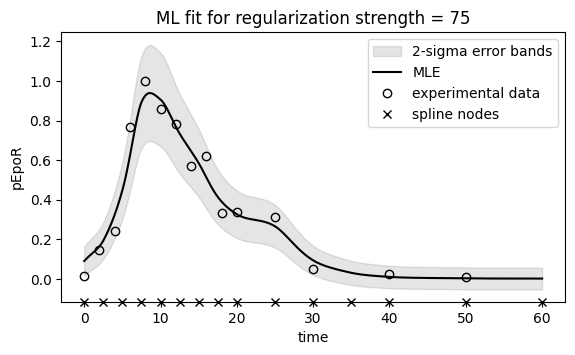
ax.set_title(f"ML fit for regularization strength = {chosen_regstrength}")
ax.legend();

# Store results for later
all_results["15 nodes, FD"] = (
    regproblems[chosen_regstrength],
    regresults[chosen_regstrength],
)

Spline approximation with few nodes, optimizing derivatives explicitly

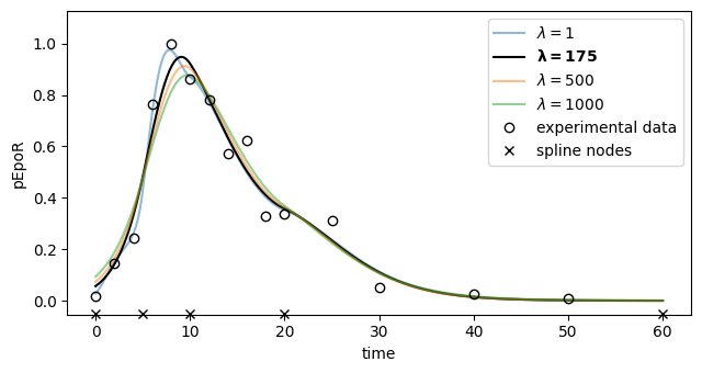
An alternative way to achieve higher expressivity, while not increasing the number of nodes, is to optimize the derivatives of the spline at the nodes instead of computing them by finite differencing. The risk of overfitting is still present, so we will include regularization as in the above example.

Creating the PEtab model

# Problem name
name = "Swameye_PNAS2003_5nodes"

We now need to create additional parameters for the spline derivatives too.

# Create spline for pEpoR
nodes = [0, 5, 10, 20, 60]
values_at_nodes = [
    sp.Symbol(f"pEpoR_t{str(t).replace('.', '_dot_')}") for t in nodes
]
derivatives_at_nodes = [
    sp.Symbol(f"derivative_pEpoR_t{str(t).replace('.', '_dot_')}")
    for t in nodes[:-1]
]
spline = amici.splines.CubicHermiteSpline(
    sbml_id="pEpoR",
    evaluate_at=amici.sbml_utils.amici_time_symbol,
    nodes=nodes,
    values_at_nodes=values_at_nodes,
    derivatives_at_nodes=derivatives_at_nodes
    + [0],  # last value is zero because steady state is reached
    extrapolate=(None, "constant"),
    bc="auto",
    logarithmic_parametrization=True,
)

# Compute L2 norm of the curvature of pEpoR
regularization = spline.squared_L2_norm_of_curvature()

# Add a parameter for regularization strength
reg_parameters_df = pd.DataFrame(
    dict(
        parameterScale="log10",
        lowerBound=1e-6,
        upperBound=1e6,
        nominalValue=1.0,
        estimate=0,
    ),
    index=pd.Series(["regularization_strength"], name="parameterId"),
)
# Encode regularization term as an additional observable
reg_observables_df = pd.DataFrame(
    dict(
        observableFormula=f"sqrt({regularization})".replace("**", "^"),
        observableTransformation="lin",
        noiseFormula="1/sqrt(regularization_strength)",
        noiseDistribution="normal",
    ),
    index=pd.Series(["regularization"], name="observableId"),
)
# and correspoding measurement
reg_measurements_df = pd.DataFrame(
    dict(
        observableId="regularization",
        simulationConditionId="condition1",
        measurement=0,
        time=0,
        observableTransformation="lin",
    ),
    index=pd.Series([0]),
)

# Add spline formula to SBML model
sbml_doc = libsbml.SBMLReader().readSBML(
    os.path.join("Swameye_PNAS2003", "swameye2003_model.xml")
)
sbml_model = sbml_doc.getModel()
spline.add_to_sbml_model(
    sbml_model, auto_add=True, y_nominal=0.1, y_constant=True
)

# Derivative parameters must be added separately
for p in derivatives_at_nodes:
    amici.sbml_utils.add_parameter(sbml_model, p, value=0.0, constant=True)

# Extra parameters associated to the spline
spline_parameters_df1 = pd.DataFrame(
    dict(
        parameterScale="log",
        lowerBound=0.001,
        upperBound=10,
        nominalValue=0.1,
        estimate=1,
    ),
    index=pd.Series(list(map(str, values_at_nodes)), name="parameterId"),
)
spline_parameters_df2 = pd.DataFrame(
    dict(
        parameterScale="lin",
        lowerBound=-0.666,
        upperBound=0.666,
        nominalValue=0.0,
        estimate=1,
    ),
    index=pd.Series(list(map(str, derivatives_at_nodes)), name="parameterId"),
)

# Create PEtab problem
petab_problem = petab.Problem(
    sbml_model,
    condition_df=petab.conditions.get_condition_df(
        os.path.join("Swameye_PNAS2003", "swameye2003_conditions.tsv")
    ),
    measurement_df=petab.core.concat_tables(
        [
            os.path.join("Swameye_PNAS2003", "swameye2003_measurements.tsv"),
            reg_measurements_df,
        ],
        petab.measurements.get_measurement_df,
    ).reset_index(drop=True),
    parameter_df=petab.core.concat_tables(
        [
            os.path.join("Swameye_PNAS2003", "swameye2003_parameters.tsv"),
            spline_parameters_df1,
            spline_parameters_df2,
            reg_parameters_df,
        ],
        petab.parameters.get_parameter_df,
    ),
    observable_df=petab.core.concat_tables(
        [
            os.path.join("Swameye_PNAS2003", "swameye2003_observables.tsv"),
            reg_observables_df,
        ],
        petab.observables.get_observable_df,
    ),
)

# Check whether PEtab model is valid
assert not petab.lint_problem(petab_problem)

# Save PEtab problem to disk
# import shutil
# shutil.rmtree(name, ignore_errors=True)
# os.mkdir(name)
# petab_problem.to_files_generic(prefix_path=name)

Creating the pyPESTO problem

# Problem must be "flattened" to be used with AMICI
petab.core.flatten_timepoint_specific_output_overrides(petab_problem)

# Check whether simulation from the PEtab problem works
# import amici.petab_simulate
# simulator = amici.petab_simulate.PetabSimulator(petab_problem)
# simulator.simulate(noise=False)

# Import PEtab problem into pyPESTO
pypesto_problem = pypesto.petab.PetabImporter(
    petab_problem, model_name=name
).create_problem()

Maximum Likelihood estimation

# Try different regularization strengths
regstrengths = np.asarray([1, 175, 500, 1000])
if os.getenv("GITHUB_ACTIONS") is not None:
    regstrengths = np.asarray([175])
regproblems = {}
regresults = {}

for regstrength in regstrengths:
    # Fix parameter in pypesto problem
    name = f"Swameye_PNAS2003_5nodes_reg{regstrength}"
    pypesto_problem.fix_parameters(
        pypesto_problem.x_names.index("regularization_strength"),
        np.log10(
            regstrength
        ),  # parameter is specified as log10 scale in PEtab
    )
    regproblem = copy.deepcopy(pypesto_problem)

    # Load existing results if available
    if os.path.exists(f"{name}.h5"):
        regresult = pypesto.store.read_result(f"{name}.h5", problem=regproblem)
    else:
        regresult = None
    # Overwrite
    # regresult = None

    # Parallel multistart optimization with pyPESTO and FIDES
    if n_starts > 0:
        if regresult is None:
            new_ids = [str(i) for i in range(n_starts)]
        else:
            last_id = max(int(i) for i in regresult.optimize_result.id)
            new_ids = [
                str(i) for i in range(last_id + 1, last_id + n_starts + 1)
            ]
        regresult = pypesto.optimize.minimize(
            regproblem,
            n_starts=n_starts,
            ids=new_ids,
            optimizer=pypesto_optimizer,
            engine=pypesto_engine,
            result=regresult,
        )
        regresult.optimize_result.sort()
        if regresult.optimize_result.x[0] is None:
            raise Exception(
                "All multistarts failed (n_starts is probably too small)! If this error occurred during CI, just run the workflow again."
            )

    # Save results to disk
    # pypesto.store.write_result(regresult, f'{name}.h5', overwrite=True)

    # Store result
    regproblems[regstrength] = regproblem
    regresults[regstrength] = regresult

# Compute sum of squared normalized residuals
print(f"Target value is {len(df_pEpoR['time'])}")
regstrengths = sorted(regproblems.keys())
stats = []
for regstrength in regstrengths:
    t, pEpoR = simulate_pEpoR(
        N=None,
        problem=regproblems[regstrength],
        result=regresults[regstrength],
    )
    assert np.array_equal(df_pEpoR["time"], t[:-1])
    pEpoR = pEpoR[:-1]
    sigma_pEpoR = 0.0274 + 0.1 * pEpoR
    stat = np.sum(((pEpoR - df_pEpoR["measurement"]) / sigma_pEpoR) ** 2)
    print(f"Regularization strength: {regstrength}. Statistic is {stat}")
    stats.append(stat)
# Select best regularization strength
chosen_regstrength = regstrengths[
    np.abs(np.asarray(stats) - len(df_pEpoR["time"])).argmin()
]

Target value is 15
Regularization strength: 1. Statistic is 9.638207938045252
Regularization strength: 175. Statistic is 15.115255701660317
Regularization strength: 500. Statistic is 19.156287450444093
Regularization strength: 1000. Statistic is 25.09224919998158

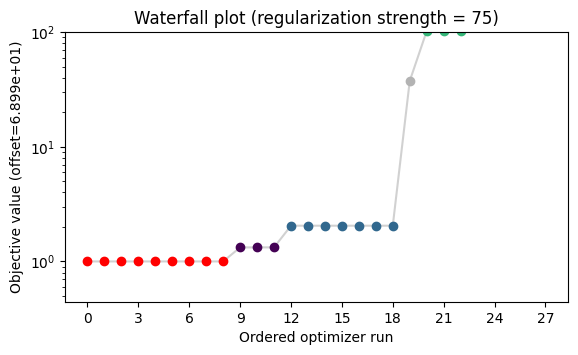
# Visualize the results of the multistarts for a chosen regularization strength
ax = pypesto.visualize.waterfall(
    regresults[chosen_regstrength], size=[6.5, 3.5]
)
ax.set_title(
    f"Waterfall plot (regularization strength = {chosen_regstrength})"
)
ax.set_ylim(ax.get_ylim()[0], 100);

# Plot ML fit for pEpoR (all regularization strengths)
fig, ax = plt.subplots(figsize=(6.5, 3.5))
for regstrength in sorted(regproblems.keys()):
    t, pEpoR = simulate_pEpoR(
        problem=regproblems[regstrength], result=regresults[regstrength]
    )
    if regstrength == chosen_regstrength:
        kwargs = dict(
            color="black",
            label=f"$\\mathbf{{\\lambda = {regstrength}}}$",
            zorder=2,
        )
    else:
        kwargs = dict(label=f"$\\lambda = {regstrength}$", alpha=0.5)
    ax.plot(t, pEpoR, **kwargs)
ax.plot(
    df_pEpoR["time"],
    df_pEpoR["measurement"],
    "o",
    color="black",
    markerfacecolor="none",
    label="experimental data",
)
ylim1 = ax.get_ylim()[0]
ax.plot(
    nodes,
    len(nodes) * [ylim1],
    "x",
    color="black",
    label="spline nodes",
    zorder=10,
    clip_on=False,
)
ax.set_ylim(ylim1, ax.get_ylim()[1])
ax.set_xlabel("time")
ax.set_ylabel("pEpoR")
ax.set_xlim(-3.0, 63.0)
ax.set_ylim(-0.05299052022388704, 1.126290214024833)
ax.legend()
ax.figure.tight_layout()
# ax.set_ylabel("input function")
# ax.figure.savefig('fit_5nodes_lambdas.pdf')

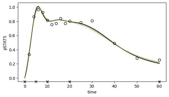
# Plot ML fit for pSTAT5 (all regularization strengths)
fig, ax = plt.subplots(figsize=(6.5, 3.5))
for regstrength in sorted(regproblems.keys()):
    t, pSTAT5 = simulate_pSTAT5(
        problem=regproblems[regstrength], result=regresults[regstrength]
    )
    if regstrength == chosen_regstrength:
        kwargs = dict(
            color="black",
            label=f"$\\mathbf{{\\lambda = {regstrength}}}$",
            zorder=2,
        )
    else:
        kwargs = dict(label=f"$\\lambda = {regstrength}$", alpha=0.5)
    ax.plot(t, pSTAT5, **kwargs)
ax.plot(
    df_pSTAT5["time"],
    df_pSTAT5["measurement"],
    "o",
    color="black",
    markerfacecolor="none",
    label="experimental data",
)
ylim1 = ax.get_ylim()[0]
ax.plot(
    nodes,
    len(nodes) * [ylim1],
    "x",
    color="black",
    label="spline nodes",
    zorder=10,
    clip_on=False,
)
ax.set_ylim(ylim1, ax.get_ylim()[1])
ax.set_xlabel("time")
ax.set_ylabel("pSTAT5");
# ax.legend();

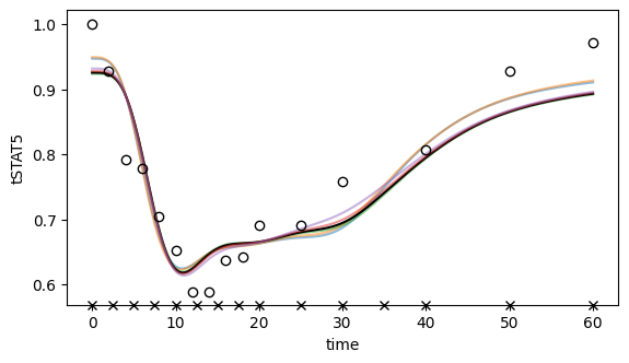
# Plot ML fit for tSTAT5 (all regularization strengths)
fig, ax = plt.subplots(figsize=(6.5, 3.5))
for regstrength in sorted(regproblems.keys()):
    t, tSTAT5 = simulate_tSTAT5(
        problem=regproblems[regstrength], result=regresults[regstrength]
    )
    if regstrength == chosen_regstrength:
        kwargs = dict(
            color="black",
            label=f"$\\mathbf{{\\lambda = {regstrength}}}$",
            zorder=2,
        )
    else:
        kwargs = dict(label=f"$\\lambda = {regstrength}$", alpha=0.5)
    ax.plot(t, tSTAT5, **kwargs)
ax.plot(
    df_tSTAT5["time"],
    df_tSTAT5["measurement"],
    "o",
    color="black",
    markerfacecolor="none",
    label="experimental data",
)
ylim1 = ax.get_ylim()[0]
ax.plot(
    nodes,
    len(nodes) * [ylim1],
    "x",
    color="black",
    label="spline nodes",
    zorder=10,
    clip_on=False,
)
ax.set_ylim(ylim1, ax.get_ylim()[1])
ax.set_xlabel("time")
ax.set_ylabel("tSTAT5");
# ax.legend();

# Plot ML fit for pEpoR (single regularization strength with noise model)
fig, ax = plt.subplots(figsize=(6.5, 3.5))
t, pEpoR = simulate_pEpoR(
    problem=regproblems[chosen_regstrength],
    result=regresults[chosen_regstrength],
)
sigma_pEpoR = 0.0274 + 0.1 * pEpoR
ax.fill_between(
    t,
    pEpoR - 2 * sigma_pEpoR,
    pEpoR + 2 * sigma_pEpoR,
    color="black",
    alpha=0.10,
    interpolate=True,
    label="2-sigma error bands",
)
ax.plot(t, pEpoR, color="black", label="MLE")
ax.plot(
    df_pEpoR["time"],
    df_pEpoR["measurement"],
    "o",
    color="black",
    markerfacecolor="none",
    label="experimental data",
)
ylim1 = ax.get_ylim()[0]
ax.plot(
    nodes,
    len(nodes) * [ylim1],
    "x",
    color="black",
    label="spline nodes",
    zorder=10,
    clip_on=False,
)
ax.set_ylim(ylim1, ax.get_ylim()[1])
ax.set_xlabel("time")
ax.set_ylabel("pEpoR")
ax.set_title(f"ML fit for regularization strength = {chosen_regstrength}")
ax.legend();

# Store results for later
all_results["5 nodes"] = (
    regproblems[chosen_regstrength],
    regresults[chosen_regstrength],
)

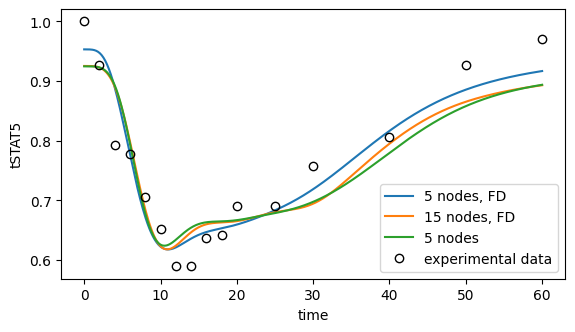
Comparing the three approaches

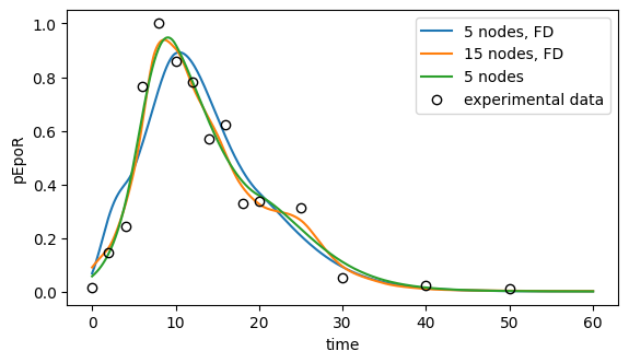
# Plot ML fit for pEpoR
fig, ax = plt.subplots(figsize=(6.5, 3.5))
for label, (problem, result) in all_results.items():
    t, pEpoR = simulate_pEpoR(problem=problem, result=result)
    ax.plot(t, pEpoR, label=label)
ax.plot(
    df_pEpoR["time"],
    df_pEpoR["measurement"],
    "o",
    color="black",
    markerfacecolor="none",
    label="experimental data",
)
ax.set_xlabel("time")
ax.set_ylabel("pEpoR")
ax.legend();

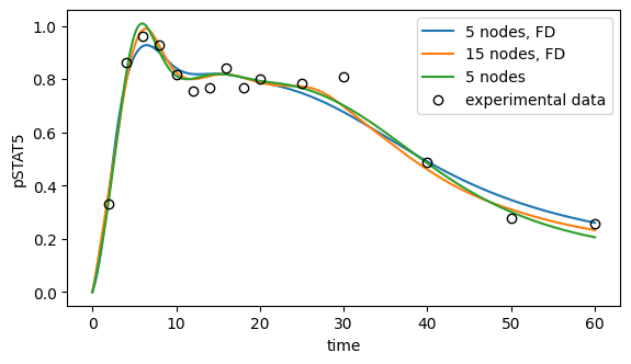
# Plot ML fit for pSTAT5
fig, ax = plt.subplots(figsize=(6.5, 3.5))
for label, (problem, result) in all_results.items():
    t, pSTAT5 = simulate_pSTAT5(problem=problem, result=result)
    ax.plot(t, pSTAT5, label=label)
ax.plot(
    df_pSTAT5["time"],
    df_pSTAT5["measurement"],
    "o",
    color="black",
    markerfacecolor="none",
    label="experimental data",
)
ax.set_xlabel("time")
ax.set_ylabel("pSTAT5")
ax.legend();

# Plot ML fit for tSTAT5
fig, ax = plt.subplots(figsize=(6.5, 3.5))
for label, (problem, result) in all_results.items():
    t, tSTAT5 = simulate_tSTAT5(problem=problem, result=result)
    ax.plot(t, tSTAT5, label=label)
ax.plot(
    df_tSTAT5["time"],
    df_tSTAT5["measurement"],
    "o",
    color="black",
    markerfacecolor="none",
    label="experimental data",
)
ax.set_xlabel("time")
ax.set_ylabel("tSTAT5")
ax.legend();

# Compare parameter values
for label, (problem, result) in all_results.items():
    print(f"\n### {label}")
    x = result.optimize_result.x[0]
    if len(x) == len(problem.x_free_indices):
        names = problem.x_names[problem.x_free_indices]
    else:
        names = problem.x_names
    for name, value in zip(names, x):
        print(f"{name} = {value}")

### 5 nodes, FD
k1 = -0.012344171128634264
k2 = -1.11975626735931
k3 = 5.999999816644789
k4 = 0.22576351403212522
scale_tSTAT5 = -0.020792663448966672
scale_pSTAT5 = 0.1422550065768319
sigma_pEpoR_abs = -1.562249437179612
sigma_pEpoR_rel = -1.0
pEpoR_t0 = -2.6870875267006804
pEpoR_t5 = -0.7797622417853871
pEpoR_t10 = -0.11820562755751975
pEpoR_t20 = -0.9974218537437654
pEpoR_t60 = -6.90775527898212

### 15 nodes, FD
k1 = 0.1543170078851364
k2 = -1.0042579083153138
k3 = -0.17925294344845363
k4 = 0.31486258696137254
scale_tSTAT5 = -0.03364700359730668
scale_pSTAT5 = 0.11013784140762342
sigma_pEpoR_abs = -1.562249437179612
sigma_pEpoR_rel = -1.0
pEpoR_t0 = -2.40456191981547
pEpoR_t2_dot_5 = -1.6438670641678346
pEpoR_t5_dot_0 = -0.80437214623219
pEpoR_t7_dot_5 = -0.1144993579909219
pEpoR_t10_dot_0 = -0.09849380649928209
pEpoR_t12_dot_5 = -0.30861764847405077
pEpoR_t15_dot_0 = -0.535565172217061
pEpoR_t17_dot_5 = -0.8808659628360864
pEpoR_t20 = -1.1184724117332843
pEpoR_t25 = -1.3245209689075161
pEpoR_t30 = -2.3651756746835053
pEpoR_t35 = -3.4734027477458524
pEpoR_t40 = -4.578132101040909
pEpoR_t50 = -5.7968417139258435
pEpoR_t60 = -6.268875988124801
regularization_strength = 1.8750612633917

### 5 nodes
k1 = 0.2486924371230916
k2 = -0.9010429810987043
k3 = -0.3408591074551208
k4 = 0.3594353532480489
scale_tSTAT5 = -0.03395751814386045
scale_pSTAT5 = 0.1008121903144357
sigma_pEpoR_abs = -1.562249437179612
sigma_pEpoR_rel = -1.0
pEpoR_t0 = -2.8601663957890175
pEpoR_t5 = -0.7275787612811422
pEpoR_t10 = -0.08172482568007049
pEpoR_t20 = -1.02532663950965
pEpoR_t60 = -6.907755278982137
derivative_pEpoR_t0 = 0.026587630472163528
derivative_pEpoR_t5 = 0.17154606724507934
derivative_pEpoR_t10 = -0.05503215878900286
derivative_pEpoR_t20 = -0.016352876798592663
regularization_strength = 2.2430380486862944

Bibliography

Schelker, M. et al. (2012). “Comprehensive estimation of input signals and dynamics in biochemical reaction networks”. In: Bioinformatics 28.18, pp. i529–i534. doi: 10.1093/bioinformatics/bts393.

Swameye, I. et al. (2003). “Identification of nucleocytoplasmic cycling as a remote sensor in cellular signaling by databased modeling”. In: Proceedings of the National Academy of Sciences 100.3, pp. 1028–1033. doi: 10.1073/pnas.0237333100.